Toxics Release Analysis in R
Federal and state environmental protection agencies monitor and regulate the release of toxins into the environment. They also evaluate the toxic legacies of abandoned industrial sites (brownfields) and, in some cases, assist in the remediation of those sites so they can be returned to productive uses.
US facilities in different industry sectors are required by law to report to the US EPA annually the quantities of chemicals that they release into the environment (air, water, or land disposal) and/or manage through recycling, energy recovery and treatment.
The Toxics Release Inventory (TRI) is a compilation by the US EPA of reported toxic chemicals that may pose a threat to human health and the environment. The TRI is intended support informed decision-making by companies, government agencies, non-governmental organizations and the public.
This tutorial covers analysis of TRI data in the US state of Illinois relative to demographics and cancer rates.
Acquire the Data
EPA Toxics Release Inventory
The US EPA's Toxics Release Inventory (TRI) is program that collects information reported annually by U.S. facilities in different industry sectors annually quantities of toxic chemical released to the air, water, or land disposal, and/or managed through recycling, energy recovery and treatment. The TRI was created by section 313 of the Emergency Planning and Community Right-to-Know Act (EPCRA) of 1986 (EPA 2021).
Summary "basic data files" can be download for individual states from the EPA TRI basic data files page.
This tutorial uses the 2019 file for the state of Illinois, which includes the latitudes and longitudes of reporting facilities, along with multiple rows for each facility describing separate groups of chemicals and the estimated quantities of releases.
Cancer and Demographic Data
A copy of the demographic and cancer data used in this tutorial is available here.
- Cancer data for this tutorial was originally sourced from the Illinois State Cancer Registry.
- Demographic data for this tutorial was originally sourced from the American Community Survey 2015-2019 five-year estimates.
- Download and processing of this data is described in the tutorial Cancer Data Analysis in R.

Process the Data
Load Demographic and Cancer Data
The precompiled data file above can be loaded with the st_read() function from the Simple Features library.
library(sf)

zip.codes = st_read("2021-minn-all-cancers.geojson")
The resulting object is a simple features polygon data frame with demographic and cancer incidence data by ZIP Code in Illinois. Of the numerous fields, the following fields are use in this tutorial:
- Estimated.Rate: Crude cancer rate per 100k per year for all cancers
- Age.Adjusted.Rate: An estimate of the age-adjusted rate based on regression of crude rates and median age
- geometry: Simple features polygon geometry
Load the Toxic Release Inventory Basic Data
The toxic release data is a CSV file that can be imported with the read.csv() function.
tri = read.csv("tri_2019_il.csv", as.is=T)

names(tri)

	  [1] "X1..YEAR"                        "X2..TRIFD"
	  [3] "X3..FRS.ID"                      "X4..FACILITY.NAME"
	  [5] "X5..STREET.ADDRESS"              "X6..CITY"
	  [7] "X7..COUNTY"                      "X8..ST"
	  [9] "X9..ZIP"                         "X10..BIA"
	 [11] "X11..TRIBE"                      "X12..LATITUDE"
	 [13] "X13..LONGITUDE"                  "X14..HORIZONTAL.DATUM"
	 [15] "X15..PARENT.CO.NAME"             "X16..PARENT.CO.DB.NUM"
	 [17] "X17..STANDARD.PARENT.CO.NAME"    "X18..FEDERAL.FACILITY"
	 [19] "X19..INDUSTRY.SECTOR.CODE"       "X20..INDUSTRY.SECTOR"
		...
Because the columns have numbered names, the names brought in by read.csv() are a bit unweildy. They can be modified with regular expressions using gsub().
names(tri) = gsub("X\\d+\\.\\.", "", names(tri))

names(tri) = gsub("[0-9\\d\\.ABCD]+\\.\\.\\.", "", names(tri))

names(tri)

	  [1] "YEAR"                       "TRIFD"
	  [3] "FRS.ID"                     "FACILITY.NAME"
	  [5] "STREET.ADDRESS"             "CITY"
	  [7] "COUNTY"                     "ST"
	  [9] "ZIP"                        "BIA"
	 [11] "TRIBE"                      "LATITUDE"
	 [13] "LONGITUDE"                  "HORIZONTAL.DATUM"
	 [15] "PARENT.CO.NAME"             "PARENT.CO.DB.NUM"
	 [17] "STANDARD.PARENT.CO.NAME"    "FEDERAL.FACILITY"
	 [19] "INDUSTRY.SECTOR.CODE"       "INDUSTRY.SECTOR"
		...
Each row in the TRI data frame represents a single type of emission from each facility. Because facilities can release multiple chemicals, one facility can have multiple rows.
For our purposes, we will use these fields:
- FACILITY.NAME: Name of the facility
- CITY: Name of facility location city in Illinois
- LATITUDE: Latitude of the facility
- LONGITUDE: Longitude of the facility
- CARCINOGEN: Whether the release is a carcinogen ("YES" or "NO")
- FUGITIVE.AIR: Amount of chemical released due to leaks of gases or vapors from pipes and containers
- STACK.AIR: Amount of the chemical released through smokestack emissions
- WATER: Amount of the chemical released into surface water
- UNIT.OF.MEASURE: The unit of measurement for the release amounts given above ("Pounds" or "Grams")
Convert to Pounds
Some values are given in grams rather than pounds. We convert those rows to pounds to make it possible to sum them together with other rows.
multiplier = ifelse(tri$UNIT.OF.MEASURE == "Grams", 1 / 453.592, 1)

tri$FUGITIVE.AIR = multiplier * tri$FUGITIVE.AIR

tri$STACK.AIR = multiplier * tri$STACK.AIR

tri$WATER = multiplier * tri$WATER

tri$UNIT.OF.MEASURE = "Pounds"
Create Overall Sums
To make it possible to total values across the whole data frame, we set any missing (NA) values to zero.
tri$FUGITIVE.AIR[is.na(tri$FUGITIVE.AIR)] = 0

tri$STACK.AIR[is.na(tri$STACK.AIR)] = 0

tri$WATER[is.na(tri$WATER)] = 0

tri$TOTAL.POUNDS = tri$FUGITIVE.AIR + tri$STACK.AIR + tri$WATER

tri$CARCINOGEN.POUNDS = ifelse(tri$CARCINOGEN == "YES", tri$TOTAL.POUNDS, 0)
Convert the Rows to Spatial Points
The data includes latitudes and longitudes for the locations, which can be converted to spatial features points using the st_as_sf() function.
library(sf)

tri = st_as_sf(tri, coords = c("LONGITUDE", "LATITUDE"), crs = 4326)
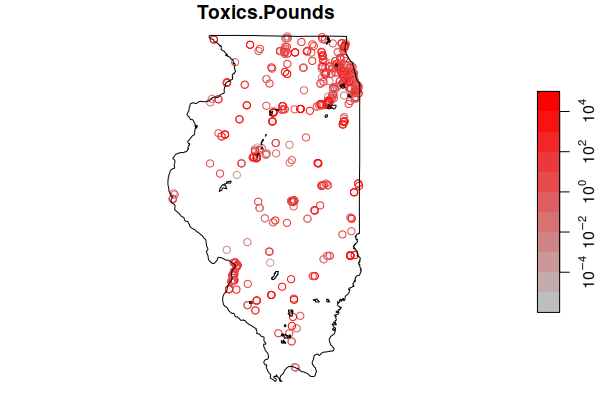
These can now be mapped with plot(). Although the map clearly shows the bulk of the sites around Chicagoland, there are facilities emitting carcinogens in all populated areas around the state.
- The reset=F parameter tells the plot() function not to reset the drawing coordinates so they can be used by the next plot on top of the map.
- In order to provide geographic context, we plot() the ACS ZIP Code st_geometry() of all ZIP Codes blended together with st_union() to show the outline of the state.
- The add=T parameter indicates to plot() on top of whatever is on the screen, without clearing the screen.
plot(tri["CARCINOGEN.POUNDS"], logz=T, pal=colorRampPalette(c("navy", "lightgray", "red")), reset=F)

plot(st_geometry(st_union(zip.codes)), add=T)

Estimate Exposure by ZIP Code
For the purposes of this simplified exploratory example, we use a simple distance decay model that assumes that amount of exposure in a ZIP Code to a toxic release is proportional to the inverse of the distance from the release source to the center of the ZIP Code.
This operates on an assumption that toxics disperse evenly around the facility and that all different carcinogens are equally carcinogenic. If more rigor is needed, a transport model should be developed to model wind and water flow patterns and how they transport the toxics. These models can be quite complex (Beyea and Hatch 1999).
- st_distance() creates a matrix of distances from ZIP Code to each toxics release source in meters.
- The weight_matrix is calculated by taking the inverse of the values in the distance matrix. The meters in the matrix are divided by an (arbitrary) 100 to get tenths of kilometers that seem to give reasonable results. One is added to prevent a divide by zero if a release source is zero kilometers from the ZIP Code.
- The source release amounts are multipled by the weights, with the columns summed to give the amount of exposure in each ZIP Code.
distance_matrix = st_distance(tri, st_centroid(zip.codes))

units(distance_matrix) = NULL

weight_matrix = 1 / (1 + (distance_matrix / 100))

zip.codes$Total.Pounds = colSums(tri$TOTAL.POUNDS * weight_matrix)

zip.codes$Carcinogen.Pounds = colSums(tri$CARCINOGEN.POUNDS * weight_matrix)

zip.codes$Fugitive.Air = colSums(tri$FUGITIVE.AIR * weight_matrix)

zip.codes$Stack.Air = colSums(tri$STACK.AIR * weight_matrix)

zip.codes$Water = colSums(tri$WATER * weight_matrix)
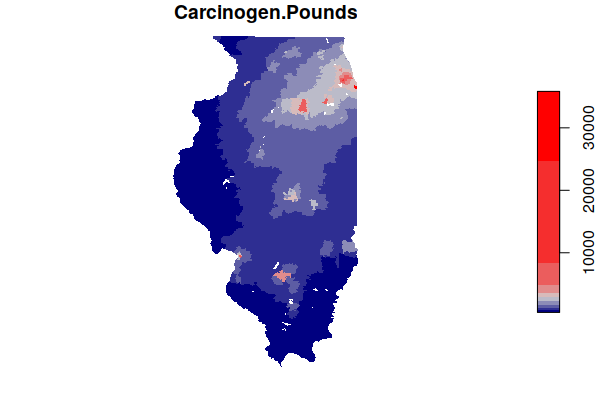
Mapping the carcinogen releases, we see effectively see a heat map of highlighting major industrial agglomerations in Illinois, notably along the Illinois River southwest of Chicago.
plot(zip.codes["Carcinogen.Pounds"], border=NA, breaks="jenks",
	pal=colorRampPalette(c("navy", "lightgray", "red")))

Save a GeoJSON File
It may be helpful to save this processed data to a GeoJSON file in case you need it in the future and either can't get the original data files or don't want to re-run all the processing steps.
st_write(zip.codes, "2021-minn-toxics-zip.geojson", delete_dsn=T)
st_write(tri, "2021-minn-toxics-facilities.geojson", delete_dsn=T)
Analyze the Data
Distribution
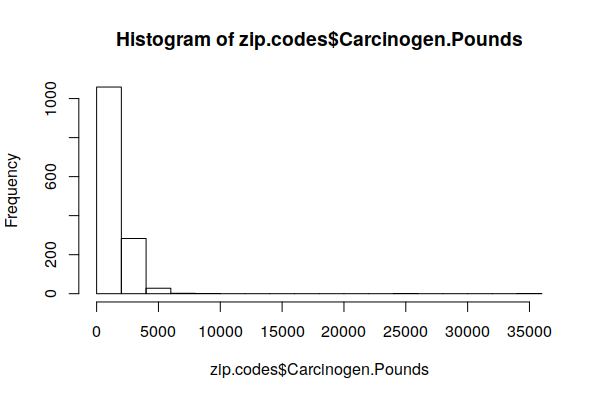
The histogram of the distribution shows that most counties are exposed to very low carcinogen releases.
hist(zip.codes$Carcinogen.Pounds, breaks=20)

Because the distribution is heavily skewed, the mean() is not relevant. The quantile() shows that, with this model, half of all ZIP Codes are exposed to 1/2 ton or less and 75% are exposed to less than one ton.
print(round(quantile(zip.codes$Carcinogen.Pounds, na.rm=T)))

   0%   25%   50%   75%  100%
  447   904  1164  1881 35828
Top ZIP Codes
By sorting the data in decreasing order() of emissions, we can see the top six ZIP Codes are each exposed to many tons of carcinogenic releases.
These highly localized areas of high releases are also visible on the map above.
zip.codes = zip.codes[order(zip.codes$Carcinogen.Pounds, decreasing=T),]

head(st_drop_geometry(zip.codes[,c("Name", "Carcinogen.Pounds")]))

	     Name Carcinogen.Pounds
	308 60633         35827.723
	221 60501         24646.025
	905 62084          8324.801
	338 60804          7036.734
	312 60638          6553.254
	246 60534          5891.762
	856 62526          33914.47
Top Sources
The list of facilities can be ordered to list the top emmiters of toxics and the top emmitters of carcinogens.
tri = tri[order(tri$CARCINOGEN.POUNDS, decreasing=T),]

head(st_drop_geometry(tri[, c("FACILITY.NAME", "CITY", "CARCINOGEN.POUNDS")]), n=10)

				FACILITY.NAME         CITY CARCINOGEN.POUNDS
	3725              TATE & LYLE DECATUR      DECATUR             91887
	776          INGREDION INC ARGO PLANT BEDFORD PARK             85891
	439  SABIC INNOVATIVE PLASTICS US LLC       OTTAWA             83393
	438  SABIC INNOVATIVE PLASTICS US LLC       OTTAWA             78414
	188                 SWAN SURFACES LLC    CENTRALIA             56900
	1993              WOOD RIVER REFINERY       ROXANA             41861
To get more details on carcinogens from a specific facility, you can subset based on the name.
print(tri[(tri$FACILITY.NAME == "INGREDION INC ARGO PLANT") &
	(tri$CARCINOGEN == "YES"), c("CHEMICAL", "CARCINOGEN.POUNDS")])

				    CHEMICAL CARCINOGEN.POUNDS
	776                     Acetaldehyde      8.589100e+04
	770 Dioxin and dioxin-like compounds      9.184465e-04
Correlations
An initial investigation of relationships often starts by looking for correlations.
First, we filter only the numeric variables in the ZIP Code data set. We also remove the margin of error (MOE) variables and remove the geometry information so we are left with a table of numeric values.
numerics = Filter(is.numeric, zip.codes)

numerics = numerics[,!grepl("MOE", names(numerics))]

numerics = st_drop_geometry(numerics)
Next we use the cor() function to find correlations with the estimated cancer rate in each ZIP Code. As might be expected with cancer, the strongest correlations are variables associated with high or low numbers of older residents who are at higher risk for cancer.
correlations = cor(numerics$Estimated.Rate, numerics, use="pairwise.complete.obs")

correlations = t(round(correlations, 3))

correlations = correlations[order(correlations, decreasing=T),]

print(head(correlations, n=10))

		     Estimated.Rate                  Median.Age
			      1.000                       0.487
		    Percent.65.Plus    Old.age.Dependency.Ratio
			      0.451                       0.414
			 Crude.Rate           Age.Adjusted.Rate
			      0.412                       0.407
	       Age.Dependency.Ratio          Percent.Homeowners
			      0.324                       0.301
	Percent.Drove.Alone.to.Work            Percent.Disabled
			      0.288                       0.278


print(tail(correlations, n=10))

	Average.Household.Size       Total.Households    Pop.per.Square.Mile
			-0.334                 -0.341                 -0.343
	Grad.School.Enrollment        K.12.Enrollment       Total.Population
			-0.356                 -0.360                 -0.369
	  Undergrad.Enrollment   Percent.Foreign.Born     Enrolled.in.School
			-0.382                 -0.383                 -0.403
	   Women.Aged.15.to.50
			-0.412
In looking specifically at the correlation between both estimated crude rates and age-adjusted rates and carcinogenic releases by ZIP Code, we find a negative correlation, which counterintuitively indicates that areas with more carcinogenic releases actually have lower crude cancer rates and similar age-adjusted rates compared to cleaner areas.
cor(zip.codes$Carcinogen.Pounds, zip.codes$Estimated.Rate, use="pairwise.complete.obs")

	[1] -0.2224945

cor(zip.codes$Carcinogen.Pounds, zip.codes$Age.Adjusted.Rate, use="pairwise.complete.obs")

	[1] -0.01146388
Multiple Regression
One way to try to tease out the interrelationships between these variables is the use of multiple regression, which creates a model that considers multiple explanatory (independent) variables to predict the outcome of a response (dependent) variable.
Multiple regression can be considered a form of supervised machine learning where you provide a set of variables that determine the model output, and let the software (machine) figure out the relationship between them that best fits the training data.
For example, this code models crude rates for all types of cancer combined as a function of median age, median household income, and carcinogen release exposure.
- The lm() (linear model) function takes a formula, which is the dependent variable (Estimate.Rate), followed by a tilde (~), and then the independent variables added together.
- The data parameter specifies the data frame from which the variables will be drawn (the training data).
model = lm(Estimated.Rate ~ Median.Age + Percent.Foreign.Born +
	Median.Household.Income + Carcinogen.Pounds, data=zip.codes)
The output of the summary() function describes the quality of the model.
- The R2 value indicates how well the model fits the training data on a scale of zero to one, with one being a perfect fit. It is commonly interpreted as the percent of the variance in the data that is explained by the model, with 0.28 meaning that 28% of the variation in the cancer rates can be explained by the independent variables provided to the model.
- The Pr(>|t|) probablity values beside each explanatory variable indicate the probability that any effect of this variable on the response could be attributed to randomness. Low probability values indicate higher statistical significance, and those values are flagged with multiple asterisks (***).
- The coefficient Estimate indicate how much each unit of change in the explanatory variable affects the response variable. For example, each year of change in Median.Age increases the cancer rate by 8.5 cases per 100k.
- The variable representing the level of exposure to carcinogen releases is not statistically significant. This indicates that this variable does not capture any possible effect of carcinogen release exposure on cancer rates.
- The R2 value of 0.325 indicates that the model accounts for around 33% of the variation in cancer rates.
print(summary(model))

	Call:
	lm(formula = Estimated.Rate ~ Median.Age + Percent.Foreign.Born +
	    Median.Household.Income + Carcinogen.Pounds, data = zip.codes)

	Residuals:
	    Min      1Q  Median      3Q     Max
	-435.22  -67.92    1.59   64.08  410.51

	Coefficients:
				  Estimate Std. Error t value Pr(>|t|)
	(Intercept)              3.195e+02  2.164e+01  14.764  < 2e-16 ***
	Median.Age               8.535e+00  4.683e-01  18.227  < 2e-16 ***
	Percent.Foreign.Born    -3.545e+00  4.015e-01  -8.829  < 2e-16 ***
	Median.Household.Income -3.336e-04  1.246e-04  -2.677  0.00752 **
	Carcinogen.Pounds       -2.354e-03  2.209e-03  -1.065  0.28693
	---
	Signif. codes:  0 ‘***’ 0.001 ‘**’ 0.01 ‘*’ 0.05 ‘.’ 0.1 ‘ ’ 1

	Residual standard error: 105.2 on 1330 degrees of freedom
	  (40 observations deleted due to missingness)
	Multiple R-squared:  0.3253,    Adjusted R-squared:  0.3232
	F-statistic: 160.3 on 4 and 1330 DF,  p-value: < 2.2e-16
Spatial Lag Regression
One of the major issues with using multiple regression with geospatial data is that the ordinary least squares algorithm used to build the model assumes that the variables are not autocorrelated, meaning that that there is no correlation between a sequence of values at different parts of the distribution.
Geographical phenomena are very commonly clustered together in space, which means that geospatial variables very commonly exhibit autocorrelation that causes multiple regression model coefficients and outputs to be biased so the model outputs are untrustworthy.
One technique for addressing this issue is spatial lag regression that performs multiple regression modeling in a way that compensates for clustering of similar values across neighboring areas (spatial lag).
- The functions for spatial regression are in the spdep library.
- Prior to performing spatial lag regression, you need to create a matrix of neighbors using the dnearneigh() function and a list of weights using the nb2listw() function.
- The lagsarlm() function performs the regression. The first parameter is a model specified in the same way as with lm(). The additional parameters (including the list of weights) are specific to spatial lag regression.
- The lag parameter is Rho, which is fairly large (0.28023). The low p-value (5.2207e-06) indicates that spatial autocorrelation is significant and is accounted for by the model.
- Notably, median household income, which was significant in the multiple regression model above, is no longer significant when spatial lag is considered.
library(spdep)

neighbors = dnearneigh(as_Spatial(st_centroid(zip.codes)), d1 = 0, d2 = 30)

weights = nb2listw(neighbors, zero.policy=T)

model = lagsarlm(Estimated.Rate ~ Median.Age + Percent.Foreign.Born +
	Median.Household.Income + Carcinogen.Pounds,
	data=zip.codes, listw=weights, tol.solve=1.0e-30, zero.policy=T)

summary(model)

	Call:lagsarlm(formula = Estimated.Rate ~ Median.Age + Percent.Foreign.Born +
	    Median.Household.Income + Carcinogen.Pounds, data = zip.codes,
	    listw = weights, zero.policy = T, tol.solve = 1e-30)

	Residuals:
	     Min       1Q   Median       3Q      Max
	-404.671  -65.148    1.680   62.854  401.244

	Type: lag
	Coefficients: (asymptotic standard errors)
				   Estimate  Std. Error z value  Pr(>|z|)
	(Intercept)              1.3273e+02  4.5391e+01  2.9242  0.003453
	Median.Age               8.2942e+00  4.6601e-01 17.7984 < 2.2e-16
	Percent.Foreign.Born    -2.8289e+00  4.3846e-01 -6.4518 1.105e-10
	Median.Household.Income -1.4350e-04  1.2872e-04 -1.1149  0.264898
	Carcinogen.Pounds       -3.1802e-04  2.2402e-03 -0.1420  0.887111

	Rho: 0.28023, LR test value: 20.755, p-value: 5.2207e-06
	Asymptotic standard error: 0.060193
	    z-value: 4.6555, p-value: 3.2313e-06
	Wald statistic: 21.674, p-value: 3.2313e-06

	Log likelihood: -8097.145 for lag model
	ML residual variance (sigma squared): 10817, (sigma: 104)
	Number of observations: 1335
	Number of parameters estimated: 7
	AIC: 16208, (AIC for lm: 16227)
	LM test for residual autocorrelation
	test value: 1.4391, p-value: 0.23029
Spatial Error Regression
A similar type of model that accounts for spatial autocorrelation is a spatial error model, which handles spatial autocorrelation as an error term in the model and improves the estimate of standard error.
- Spatial error regression is implemented in the errorsarlm(). function from the spdep library. This function uses the same parameters as the lagsarlm() function used for spatial lag regression above.
- This model gives a set of coefficients that are similar to the spatial lag model above.
- With spatial error models, the error term is Lambda. As with rho above, the high lambda (0.34119) and low p-value (3.3128e-06) indicate that spatial autocorrelation is significant in this model.
model = errorsarlm(Estimated.Rate ~ Median.Age + Median.Household.Income +
	Percent.Foreign.Born + Carcinogen.Pounds,
	data=zip.codes, listw=weights, tol.solve=1.0e-30, zero.policy=T)

summary(model)

	Call:
	errorsarlm(formula = Estimated.Rate ~ Median.Age + Median.Household.Income +
	    Percent.Foreign.Born + Carcinogen.Pounds, data = zip.codes,
	    listw = weights, zero.policy = T, tol.solve = 1e-30)

	Residuals:
	       Min         1Q     Median         3Q        Max
	-418.56991  -65.20729   -0.27079   63.65532  407.00169

	Type: error
	Coefficients: (asymptotic standard errors)
				   Estimate  Std. Error z value  Pr(>|z|)
	(Intercept)              3.2174e+02  2.1973e+01 14.6427 < 2.2e-16
	Median.Age               8.3719e+00  4.6863e-01 17.8647 < 2.2e-16
	Median.Household.Income -2.4866e-04  1.3017e-04 -1.9102   0.05611
	Percent.Foreign.Born    -3.6955e+00  4.5584e-01 -8.1069 4.441e-16
	Carcinogen.Pounds       -2.4945e-03  2.3141e-03 -1.0779   0.28107

	Lambda: 0.34119, LR test value: 21.626, p-value: 3.3128e-06
	Asymptotic standard error: 0.072435
	    z-value: 4.7103, p-value: 2.4734e-06
	Wald statistic: 22.187, p-value: 2.4734e-06

	Log likelihood: -8096.709 for error model
	ML residual variance (sigma squared): 10788, (sigma: 103.86)
	Number of observations: 1335
	Number of parameters estimated: 7
	AIC: 16207, (AIC for lm: 16227)
Principal Component Analysis
A challenge with multiple regression is that it is difficult to know which variables to include in your model, and whether the variables you have chosen give you the best model possible. In addition, if there is correlation between two or more independent variables (making them not independent), the importance of those variables to the model (as indicated by the coefficients) may be distorted (biased).
One technique for addressing that issue is principal component analysis, which uses linear algebra to reduce a matrix of all the possible variables to a smaller set of principal component variables
This reduction in the number of variables (dimensions) needed for analysis is called dimensionality reduction. Because this technique makes a determination of the importance of different variables without direct human intervention or judgement, it can also be considered a form of unsupervised machine learning.
field.complete = sapply(names(zip.codes), function(name) (sum(is.na(zip.codes[,name])) < 50))

numerics = zip.codes[,field.complete]

numerics = Filter(is.numeric, numerics)

numerics = numerics[,!grepl("MOE", names(numerics))]

numerics = st_drop_geometry(numerics)

numerics = na.omit(numerics)

numerics[,c("Percent.No.Vehicle", "Total.Count", "Crude.Rate",
	"Estimated.Rate", "Age.Adjusted.Rate",
	"Total.Pounds", "Fugitive.Air", "Stack.Air", "Water")] = NULL

pca = prcomp(numerics, scale=T)
The predict() function can be used with principal component matrix create by prcomp() and new data to create a new set of principal components. Those principal components can then be used to create a model using lm().
dependent.variable = zip.codes$Estimated.Rate

pca.data = predict(pca, st_drop_geometry(zip.codes))

pca.data = as.data.frame(pca.data)

pca.data$Estimated.Rate = dependent.variable

model = lm(Estimated.Rate ~ ., data = pca.data)

print(summary(model))

	Call:
	lm(formula = Estimated.Rate ~ ., data = pca.data)

	Residuals:
	    Min      1Q  Median      3Q     Max
	-324.74  -56.09   -2.51   53.99  392.49

	Coefficients:
		      Estimate Std. Error t value Pr(>|t|)
	(Intercept)  6.351e+02  2.540e+00 250.070  < 2e-16 ***
	PC1         -1.979e+01  7.564e-01 -26.165  < 2e-16 ***
	PC2         -1.106e+01  2.227e+00  -4.964 7.83e-07 ***
	PC3          1.151e+01  1.404e+00   8.198 5.88e-16 ***
	PC4         -2.088e+01  2.606e+00  -8.012 2.51e-15 ***
	PC5         -5.663e+00  1.776e+00  -3.189 0.001464 **
	PC6         -6.140e-01  4.877e+00  -0.126 0.899845
	PC7         -1.549e-01  4.352e+00  -0.036 0.971616
	PC8          1.564e+01  2.390e+00   6.545 8.56e-11 ***
	PC9          1.094e+01  8.165e+00   1.340 0.180555
	PC10         1.270e+00  8.052e+00   0.158 0.874736
	PC11         1.727e+01  1.912e+01   0.903 0.366500
	PC12        -4.247e+00  9.966e+00  -0.426 0.670097
	PC13        -4.048e+00  3.466e+00  -1.168 0.243092
	PC14         6.386e+00  8.466e+00   0.754 0.450813
	PC15        -1.365e+01  3.760e+00  -3.629 0.000296 ***
	PC16         2.054e+01  1.177e+01   1.746 0.081109 .
	PC17         1.439e+01  6.301e+00   2.283 0.022585 *
	PC18         2.817e+01  1.550e+01   1.817 0.069509 .
	PC19         1.276e+01  1.168e+01   1.093 0.274624
	PC20         8.240e+00  5.412e+00   1.523 0.128119
	PC21        -9.390e+00  7.160e+00  -1.311 0.189971
	PC22        -4.843e+00  4.343e+00  -1.115 0.264977
	PC23         1.261e+01  9.283e+00   1.358 0.174672
	PC24         1.418e+01  2.502e+01   0.567 0.570984
	PC25         7.404e+00  6.008e+00   1.232 0.218015
	PC26         1.333e+01  1.429e+01   0.933 0.351112
	PC27         1.360e+01  8.496e+00   1.601 0.109732
	PC28         9.290e+00  1.499e+01   0.620 0.535463
	PC29         2.299e+01  1.508e+01   1.524 0.127703
	PC30         1.093e+01  8.779e+00   1.245 0.213411
	PC31         2.107e+00  7.737e+00   0.272 0.785366
	PC32        -5.705e+00  9.134e+00  -0.625 0.532340
	PC33         1.268e+02  7.138e+01   1.776 0.075991 .
	PC34         2.588e+02  6.956e+01   3.721 0.000207 ***
	PC35        -1.121e+01  5.727e+01  -0.196 0.844839
	PC36         9.217e+01  9.737e+01   0.947 0.344025
	PC37         3.204e+02  1.250e+02   2.563 0.010495 *
	PC38         2.905e+01  2.251e+02   0.129 0.897349
	PC39        -1.021e+03  1.248e+03  -0.818 0.413434
	PC40         4.697e+03  1.140e+04   0.412 0.680427
	PC41        -2.493e+16  1.889e+16  -1.320 0.187211
	---
	Signif. codes:  0 ‘***’ 0.001 ‘**’ 0.01 ‘*’ 0.05 ‘.’ 0.1 ‘ ’ 1

	Residual standard error: 92.48 on 1284 degrees of freedom
	  (49 observations deleted due to missingness)
	Multiple R-squared:  0.4943,    Adjusted R-squared:  0.4781
	F-statistic: 30.61 on 41 and 1284 DF,  p-value: < 2.2e-16
In this case, the model built with principal components fits slightly less well than the multiple regression model (R2 of 0.741 vs 0.889), but only five components are statistically significant, so we can focus on what make up those principal components.
- PC1 is dominated by the age variables, with increased percent of older residents associated with higher rates of cancer.
- PC2 is dominated by the marriage variables, with higher rates of marriage associated with increased cancer risk and higher rates of divorce associated with lower cancer risk.
- PC3 is dominated by overall population, with higher population in a county associated with decreased cancer risk.
- PC9 is dominated by income, with higher income areas having increasing cancer risk.
- PC12 is dominated by retirement, where areas with more retirees have higher cancer risk.