Introduction to Geospatial Data in R
This tutorial will give a brief introduction on how to perform simple import and visualization of geospatial area data in R.
Installing and Using R
R is an open-source computer language and software environment for statistical analysis. R was first developed in 1993 by Ross Ihaka and Robert Gentleman at the University of Auckland, New Zealand. It based on the S statistical computing language that was originally developed at the legendary Bell Labs in 1976. R has become a popular package for data science and financial analysis.
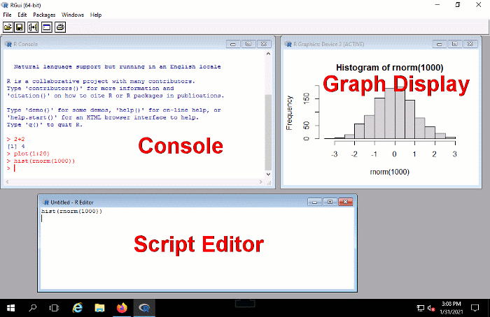
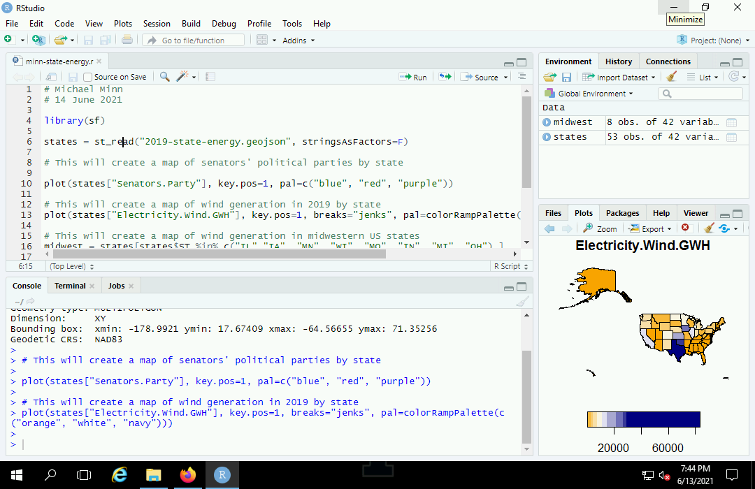
Although R on Windows has its own user interface (above), you will likely find R easier to use through the interactive development environment RStudio Desktop.
R is free, open-source software, and RStudio has a free open-source version that will likely be suitable for most users.
- If you wish to install RStudio on your personal machine, you must first download R for PC or Mac from the Comprehensive R Archive Network (CRAN) home page and install it.
- You can then download the RStudio Desktop installer.
If you are a member of the University of Illinois community, RStudio is available on most open lab computers and on computers you access remotely via UIUC AnyWare and can be found in the Start.
Language Basics
Because you interact with R almost exclusively with typed commands, you need to be familiar with some basic language elements in order to use R. While this is an unfamiliar way of working for many users and involves a learning curve, it is also a very fast and precise way of working with software once you gain a modest level of mastery of the language.
Examples in this Tutorial
In the examples given in this tutorial, commands you type are displayed preceded by a > symbol that is a prompt from the program.
After you type a command you press the Enter or Return key to execute the command.
The examples show what R will display in response to your commands.
To get the full benefit of this tutorial, it is recommended that you actually type commands into the R console as you skim through the examples.
Mathematical Expressions
At it's simplest, you can use R as a calculator and it will display the value.
2+2
	[1] 4
Mathematical expressions in R use mathematical symbols with operators (+ - * /) to calculate values. The carat operator (^) is used for exponents.
2+2
	[1] 4

10 + 2
	[1] 12

10 - 2
	[1] 8

10 * 2
	[1] 20

10 / 2
	[1] 5

10^2
	[1] 100
Objects
An object in R is a collection of one or more data values referred to by a name.
- Objects are also sometimes referred to as variables.
- Objects can be used to store the values of calculations so you can use those values in expressions later without having to repeat calculations.
- Objects also make formulas easier to read.
To display the contents of a object at the console, you simply type the name of the object.
x = 10 * 2

x
	[1] 20

x + 15
	[1] 35
R has an arrow operator (<-) that is also used to assign values to objects and you should know about this in case you look at R examples shared on the web.
The arrow assignment operator give R a distinctive look and has additional capabilities, but also makes the code more difficult for casual R users to read, so this tutorial just uses the equals sign (=) common to most other computer languages.
y <- 12 + 16

y
	[1] 28

y = 12 + 17

y
	[1] 29

12 + 18 -> y

y
	[1] 30
Object Names
Object names can contain letters, numbers, periods, and underscores (_), although they must start with a letter and are case sensitive.
hello = 12

Hello = 15

hello
	[1] 12

Hello
	[1] 15
You should always try to make your object names meaningful so that you and other people can understand what your objects are. Rather than calling a object containing a standard deviation "s" you might call it "stdev". The extra time spent typing now will save you confusion later.
Object names cannot contain spaces, but there are techniques for representing multi-word object names that get around this issue.
- wordword
- word_word (underscore)
- word.word (period)
- wordWord (camelback capitalization)
Strings
One of the most powerful features of R is that objects can contain many different types of data. Objects can also contain text.
Segments of text are called strings of characters and you create a string object by enclosing text in quotation marks.
x = "Hello"

Hello = 12

x
	[1] "Hello"

Hello
	[1] 12
Vectors
Vectors in R are collections of objects that all have the same type.
In statistical calculations, we commonly deal with groups of numbers that are thought of as a single entity, such as an attribute associated with a set of geospatial features. One of the most powerful features of R is that you can perform operations on all members of a vector with a single operation.
Vectors can be created by enclosing multiple numbers in the c() function (c is for combine).
x = c(1,3,5,7,10)

x
	[1]  1  3  5  7 10
Note that objects by default are vectors in R. If you assign a single value to an object, it is a vector of one element, which is why display of a single-valued object is preceded by a "[1]," indicating that it is the first (and only) value in the vector.
x = 20

x
	[1] 20
You can then perform multiple operations of the same kind on a vector with a single expression.
x
	[1]  1  3  5  7 10

x + 2
	[1]  3  5  7  9 12

x * 10
	[1]  10  30  50  70 100

x - 5
	[1] -4 -2  0  2  5

x / 2
	[1] 0.5 1.5 2.5 3.5 5.0

x ^ 2
	[1]   1   9  25  49 100
Built-In Functions
A function in R is a module of computer code that accomplishes a task and returns an object with the results of that task.
- In an expression, you call a function with function name, an open parenthesis, a set of zero or more parameters separated by commas, and then a closing parenthesis.
- The function then returns an object based on the parameters.
name(parameter1, parameter2, ...)
R has dozens of functions available with a default installation, and hundreds more that can be brought in from libraries that permit many different types of mathematical operations to be performed on many different types of data.
The basic descriptive statistical functions are similar to those in Excel.
x = c(2, 5, 13, 24, 35, 40, 35, 24, 13, 5,2)

x
	[1]  2  5 13 24 35 40 35 24 13  5

max(x)
	[1] 40

min(x)
	[1] 2

mean(x)
	[1] 18

median(x)
	[1] 13

sd(x) # standard deviation
	[1] 14.26184
R has functions for most common statistical operations, so analysis of data in R often simply involves finding the proper functions to use and determining what parameters those functions need.
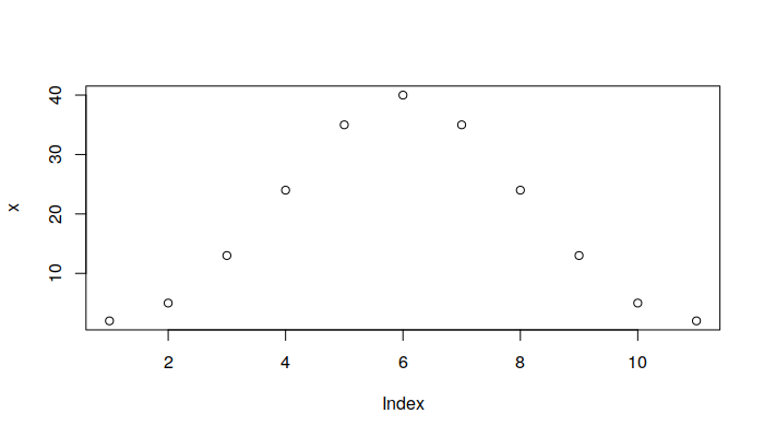
Plotting Objects
The plot() function allows you to create visualizations of objects. By default, when passed a single vector, the plot() function draws a point graph:
x = c(2, 5, 13, 24, 35, 40, 35, 24, 13, 5,2)

plot(x)
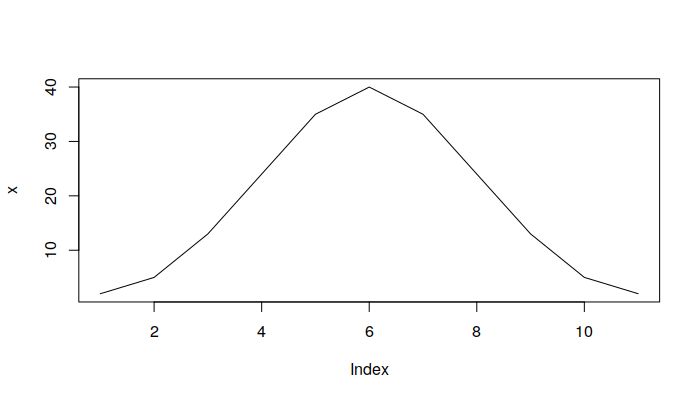
You can change that to a line graph by adding the parameter type="l":
x = c(2, 5, 13, 24, 35, 40, 35, 24, 13, 5,2)

plot(x, type="l")
Geospatial Data in R
The Simple Features Package
Geospatial data objects can be loaded from files and manipulated with functions from the Simple Features (sf) library. You may also see examples on the web using the sp package, although that package is old and hard to work with, and you should use sf for new code.
The first time you use sf on a new machine, you may need to install it first from inside R:
install.packages("sf")
Then, you load it with the library() function. This should also be at the beginning of every script you create in R that uses the sf package:
library(sf)
Loading Geospatial Data
The st_read() function will read geospatial data from most established geospatial data file formats.
For this example, we will use a GeoJSON file (2019-state-energy.geojson) of state-level energy production and consumption election data that you can download here.
states = st_read("https://michaelminn.net/tutorials/r-spatial-intro/2019-state-energy.geojson")
Reading layer `OGRGeoJSON' from data source `2019-state-energy.geojson' using driver `GeoJSON'
Simple feature collection with 3139 features and 48 fields
geometry type:  MULTIPOLYGON
dimension:      XY
bbox:           xmin: -178.9921 ymin: 18.91747 xmax: -66.9499 ymax: 71.35256
epsg (SRID):    4269
proj4string:    +proj=longlat +ellps=GRS80 +towgs84=0,0,0,0,0,0,0 +no_defs
Once you have loaded your data into an object, you can display the available geospatial attributes in the object using the names() command:
names(states)
 [1] "ST"                              "Name"
 [3] "GEOID"                           "AFFGEOID"
 [5] "Square.Miles.Land"               "Square.Miles.Water"
 [7] "State.Name"                      "Population.MM"
 [9] "Civilian.Labor.Force.MM"         "GDP.B"
[11] "GDP.Per.Capita"                  "GDP.Manufacturing.MM"
[13] "Personal.Income.Per.Capita"      "VMT.MM"
[15] "Farm.Land.MM.Acres"              "Average.Temperature"
[17] "Precipitation.Annual"            "Consumption.Coal.B.BTU"
[19] "Consumption.Jet.Fuel.B.BTU"      "Consumption.Gasoline.B.BTU"
[21] "Consumption.Total.B.BTU"         "Consumption.Per.Capita.MM.BTU"
[23] "Production.Coal.B.BTU"           "Production.Gas.B.BTU"
[25] "Production.Oil.B.BTU"            "Production.Renewable.B.BTU"
[27] "Production.Total.B.BTU"          "Electricity.Interstate.Flow.GWH"
[29] "Electricity.Average.Cost"        "Electricity.Consumption.GWH"
[31] "Electricity.Per.Capita.KWH"      "Electricity.Hydro.GWH"
[33] "Electricity.Nuclear.GWH"         "Electricity.Solar"
[35] "Electricity.Wind.GWH"            "CO2.Total.MM.Tonnes"
[37] "CO2.Per.Capita.Tonnes"           "Renewable.Standard.Type"
[39] "Renewable.Standard.Name"         "Renewable.Standard.Year"
[41] "Senators.Party"                  "geometry"
Mapping Categorical Attributes
Choropleth maps can be created from sf polygon objects with the plot() command, although you will probably need to add additional parameters to get the kind of map you are looking for.
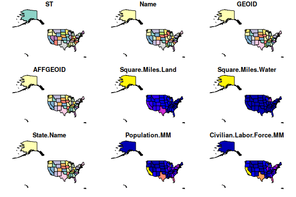
If you simply plot() the states, the plot() function will create tiny, unreadable plots of as many of the object's fields as it can fit on a plot:
plot(states)
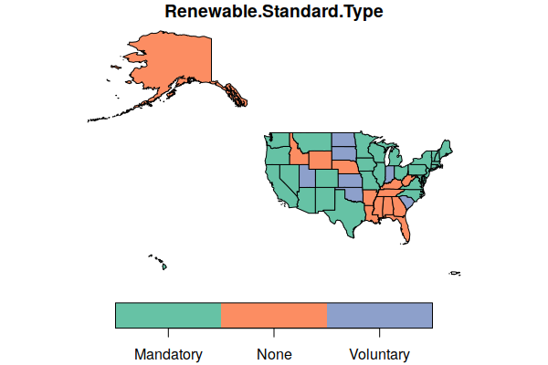
Therefore, you must select a specific field to plot() using the text name of the field to map enclosed in quotation marks (because it is text) and square brackets. In this example:
- We use the field Renewable.Standard.Type, which is the type of renewable energy standard in effect in each state.
- The key.pos=1 parameter puts the legend at the bottom rather than the side.
plot(states["Renewable.Standard.Type"], key.pos=1)
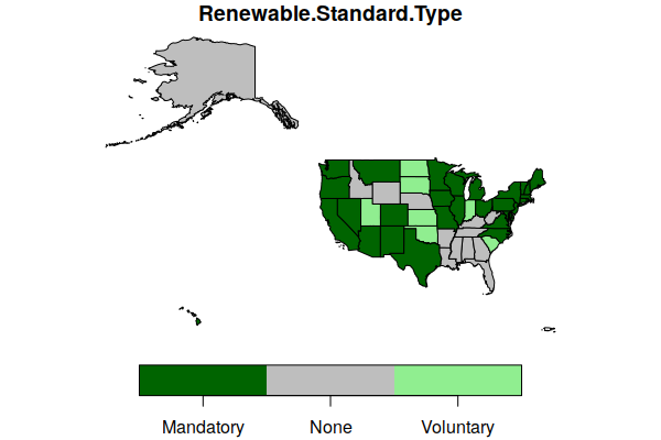
To create a map using more descriptive colors, we can pass a vector of color names to the pal (palette) parameter.
plot(states["Renewable.Standard.Type"], key.pos=1, pal=c("darkgreen", "gray", "lightgreen"))
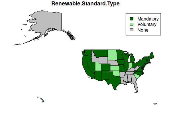
If you want a more-traditional box legend, you can use the legend() function:
- key.pos=NULL on the plot() command to turn off the default bar legend.
- x = "topright" places the legend at the top right corner of the plot.
- The legend parameter gives the names listed in the legend.
- The fill parameter gives the colors that will fill the legend color boxes.
plot(states["Renewable.Standard.Type"], key.pos=NULL, pal=c("gray", "darkgreen", "lightgreen"))

legend(x = "topright", legend=c("Mandatory", "Voluntary", "None"), fill=c("darkgreen", "lightgreen", "gray"))
Mapping Quantitative Attributes
The plot() function can be used to map quantitative attributes, although, again, you may need additional parameters to get what you want.
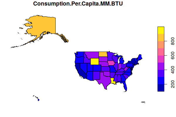
This creates a map of per-capita energy use in each state in millions of BTUs. The default plot uses a blue-purple-yellow color ramp:
plot(states["Consumption.Per.Capita.MM.BTU"])
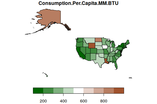
You can specify a different color ramp by passing a vector of the desired colors to the colorRampPalette() function. This example uses a diverging color scheme with a color ramp that extends from green to white to sienna (brown):
plot(states["Consumption.Per.Capita.MM.BTU"], key.pos=1,
	pal=colorRampPalette(c("darkgreen", "white", "sienna")))
Subsets
There will likely be situations where you only want to use a specific subset of a geospatial data set.
sf objects are R data frame objects that can be subsetted in the same way as other data frames.
Parts of a data frame can be defined using conditions specified inside square brackets ([]) following the name of the data frame.
As shown above, when using only one value in the square brackets, you select specific columns (fields).
To select specific rows (features), you need two values inside the brackets, separated by a comma. The first value specifies which rows (features) to select, and the second value specifies which columns to select. If you want to select all columns, you can leave the value after the column blank.
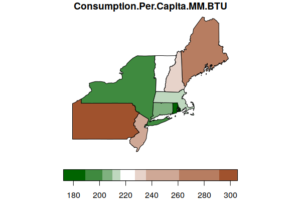
In the example below, the first value in the square brackets specifies to only select features where the ST (state abbreviation) attribute is in the vector of northeastern states.
The dollar sign (states$ST) indicates that the attribute should be drawn from the states object.
Since we want to select all columns, we just put a comma and no value before the closing square bracket.
We assign this subsetted object to a new name that we can then plot.
northeast = states[states$ST %in% c("ME", "VT", "NH", "CT", "RI", "NY", "NJ", "MA", "PA"), ]

plot(northeast["Consumption.Per.Capita.MM.BTU"], key.pos=1,
	pal=colorRampPalette(c("darkgreen", "white", "sienna")))
Projections
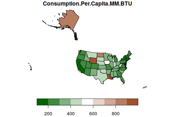
By default, the plot() function plots the geospatial data using an equirectangular projection that may be undesirable depending on what part of the world you are mapping and what you are using the map for.
The st_transform() function can be used to reproject a geospatial object to a new projection. The crs parameter will accept an EPSG number or a PROJ.4 string that describes the desired projection. For this map of the US, we use a PROJ.4 string for a Lambert conformal conic projection centered on the continental US.
lambert = "+proj=lcc +lon_0=-98 +lat_1=33 +lat_2=45"

states = st_transform(states, crs=lambert)

plot(states["Consumption.Per.Capita.MM.BTU"], key.pos=1,
	pal=colorRampPalette(c("darkgreen", "white", "sienna")))
Correlation
R is software for statistical computing, so you can perform statistical operations on geospatial data. While there are specialized functions for dealing with autocorrelation in spatial data, simple non-spatial functions can be used for data exploration.
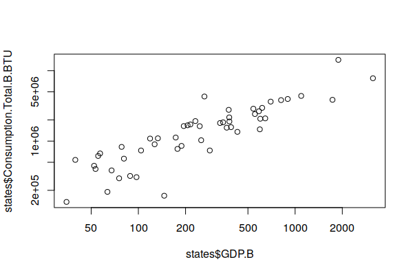
For example, there is a field for gross domestic product (GDP.B), which represents the total amount of economic activity in the state. Greater economic activity is generally associated with higher energy use. To examine whether that is true at the state level, we can plot an X/Y scatter chart between the two attributes to see if the plot shows a correlation.
For this call to plot(), we pass the two attributes. We use the dollar sign ($) to isolate individual attributes as vectors of values. To make small and large states more visible together, we use logarithmic scales for both the x and y axes (log="xy").
The chart shows a fairly clear line pattern from lower left to bottom right, indicating there is correlation.
plot(states$GDP.B, states$Consumption.Total.B.BTU, log="xy")
We can use the lm() (linear model) function to create a simple linear model and see how it fits. The tilde (~) in this function says to model one attribute in terms of the other.
R2 is the coefficient of determination that indicates the strength of correlation. The values range from zero to one, and higher values indicate stronger correlation.
The R2 value of 0.65 indicates a strong correlation, which corroborates our hypothesis that states with greater energy use generally have higher GDP.
model = lm(Consumption.Total.B.BTU ~ GDP.B, data=states)

summary(model)
Call:
lm(formula = GDP.B ~ Consumption.Total.B.BTU, data = states)

Residuals:
    Min      1Q  Median      3Q     Max
-920.53  -99.67  -41.81   35.73 1582.27

Coefficients:
                                Estimate Std. Error t value Pr(>|t|)
(Intercept)                    3.452e+01  6.019e+01   0.573    0.569
states$Consumption.Total.B.BTU 1.949e-04  2.015e-05   9.673 5.99e-13 ***
---
Signif. codes:  0 ‘***’ 0.001 ‘**’ 0.01 ‘*’ 0.05 ‘.’ 0.1 ‘ ’ 1

Residual standard error: 323.6 on 49 degrees of freedom
  (2 observations deleted due to missingness)
Multiple R-squared:  0.6563,    Adjusted R-squared:  0.6493
F-statistic: 93.58 on 1 and 49 DF,  p-value: 5.99e-13
Scripts
Another powerful advantage of a command-line console is that you can type commands into script files and run them. This makes it possible to easily repeat complex sequences of operations. And if you find an error in your script, you can fix it and rerun the script without the labor of having to repeat long sequences of button clicks that you would need when using software with a graphical user interface like ArcGIS Pro.
This video demonstrates the creation of a script in RStudio with code chunks from the tutorial above to analyze the relationship between total energy consumption and GDP at the state level.
- Create a new project from File, New Project, and New Directory and give the directory a meaningful name that will help you remember what the project is about.
- Create a new script from File, New File, R Script.
- Click the Save icon and save the script to a meaningfully named file. If you are only planning on having one script in the project, it can be helpful to just use the same name as the project.
- Add chunks of code with comments explaining what the code does. Comments are useful to help you remember what the code does and for other people that may need to use or modify your code.
- When you are done, run your full script to make sure it completes with no errors.
- You can view the plots generated by your code in the Plots window.
- Make sure all files are saved by selecting File and Save All.
Comments
Comments in scripts are lines that the program ignores. These lines are used for documenting the authorship of scripts and for adding comments that explain what is going on when you have complex sequences of expressions and function calls.
Comments start with a pound sign (#) and tell the R interpreter to ignore everything that follows on that line.
# Name of script (date)
# This is a comment that explains what the line after it does

x = 2 + 2
Getting Help
From within the R console, you can get documentation for most functions by typing a question mark followed by the name of the function. Type:
?mean
If you have only a vague idea of what you want, you can type a double question mark and a keyword. Type:
??normal
If you have any more complex questions about the language syntax or a cryptic error message issued by the program, there is a vast amount of R information on a variety of Internet websites. The Google is your tech support for R.