Markdown Notebooks in R

One challenge with using scripting languages for complex analysis is maintaining the relationship between the code used to perform the analysis and the descriptive text and imagery used to explain the outputs of that code to the intended audience of the analysis.

While you can collect your R code in scripts of R code and use comments to explain what you are doing, scripts must be run in the software to create output graphics, and most non-programmers cannot meaningfully read scripts anyway. Long blocks of code in scripts can even be difficult to decipher by other people who want to reuse or modify your code.

One common contemporary solution to this challenge is the use of notebooks that integrate code, visualizations, and descriptive text together into unified documents. Notebooks can then be rendered to documents in a variety of different formats that you can share with collaborators or audience members. The documents rendered from notebooks can also be used as a quick way to export graphics from R that can then be copied into other materials like web pages or posters.

RStudio provides a notebook interface to work with documents that have been prepared in the R Markdown format.

This tutorial describes basics for creating notebooks in R and exporting to a MS Word document that can be shared with your audience.

Installing rmarkdown

To use notebooks in RStudio, you will need the rmarkdown package.

For these geospatial examples, you will also need the sf package.

You can install this package using the Tools -> Install Packages... dialog in RStudio, or issue the install.packages commands from a console.

> install.packages('rmarkdown')

Installing rmarkdown in RStudio

Starting a Notebook

If you haven't created your project already, create a new project with File, New Project, and New Directory. Use a meaningful name so that you will remember what the project contains when you see this directory in the future.

Start a new notebook with File -> New File -> R Notebook. This will create a bare-bones notebook with boilerplate text that you should modify.

Click the Save icon to save your notebook under a meaningful name with the .Rmd extension.

The first four lines are a metadata header that indicate the title (printed at the top of your report) and the output format. The "---" delimiters indicate the start and end of the header, so you should leave them alone.

---
title: "R Notebook"
output: html_notebook
---

You should change the title as needed, but the output format can be left alone since it will be automatically modified by the software when you render your notebook to an output file. You may also consider adding author and date entries.

---
title: "Median Household Income in Illinois"
author: "Michael Minn"
date: "16 June 2021"
output: html_notebook
---

Creating a new notebook in RStudio

Error Saving File

If you get an Error Saving File message of The filename, directory name, or volume label syntac is incorrect when you try to save your .Rmd file, and if you are on a networked machine (like SESE-GIS or AnyWare), your working directory may be on a networked file system, which confuses RStudio.

Set Working Directory -> Choose Directory... and use a directory under a file letter (like u:) rather than one of the This PC directories.

Upload Data

The examples in this tutorial use a GeoJSON file of commonly-used county-level variables from the 2015-2019 American Community Survey five-year estimates from the US Census Bureau.

This video demonstrates how to download a data file to your local machine and then upload it into your RStudio project directory.

You can download the data and view the metadata here.

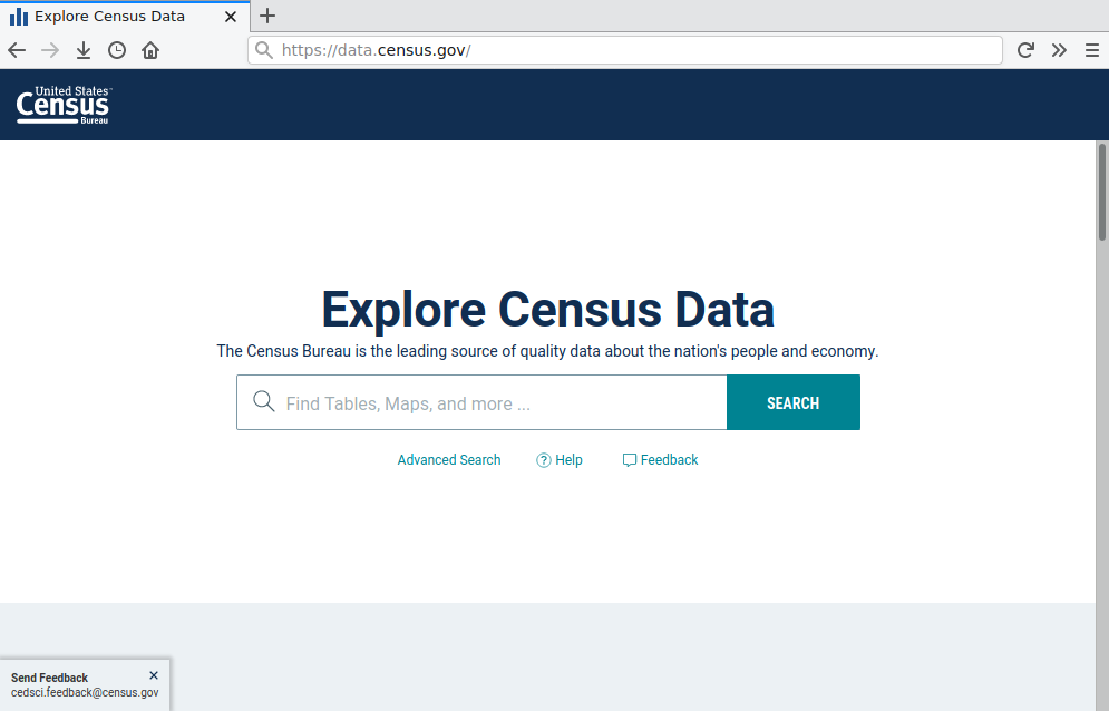
Uploading data into an RStudio project

You can download US Census Bureau data directly from data.census.gov, but that data requires extensive additional processing to be mapped as a choropleth. Those procedures are described in the tutorial Importing US Census Bureau Data into R.

Inline Text

Following the metadata is some sample inline text that will be rendered to your document as text rather than executed as R code.

You can delete this example text and replace it with something more appropriate.

---
title: "Median Household Income in Illinois"
author: "Michael Minn"
date: "16 June 2021"
output: html_notebook
---

This document describes the distribution of median household income
around the state of Illinois based on data from the US Census Bureau's
2015-2019 American Community Survey five-year estimates.

Formatting Elements

There are a variety of formatting elements you can add to your text if needed. Some commonly used elements include:

To start a new paragraph, enter a blank line between blocks of text.
To italicize text, surround your text with asterisks: *text*
To bold text, surround your text with double asterisks: **text**
To create subscripts, surround your text with tildes: CO~2~
To create superscripts, surround your text with carats: R^2^

For example:

Former vice-president Al Gore's 2006 concert/documentary film 
*An Inconvenient Truth* on the climate change challenges posed 
by rising CO~2~ levels grossed $24 million in the US (Wikipedia 2021).

Would be rendered as:

Former vice-president Al Gore's 2006 concert/documentary film An Inconvenient Truth on the climate change challenges posed by rising CO₂ levels grossed $24 million in the US (Wikipedia 2021).

Other formatting options are described in the R Markdown documentation.

Adding and Previewing Code Chunks

Chunks of R code are included in notebooks between lines that open with the delimiter "```{r}" and close with the delimiter "```"

Note that these are back ticks that are usually on the same key with the tilde (~) on US computer keyboards.

Maps

The following code loads the demographic data file (described above) and creates a choropleth of median household income by county in the US.

A choropleth is a type of thematic map where areas are colored or textured based on some data variable.

breaks="quantile" distributes the colors evenly over the range of values.
border=NA parameter turns off the borders so they don't obscure small counties.
key.pos=1 places the legend at the bottom of the map to make it easier to read and to use space more efficiently.

```{r}
library(sf)

counties = st_read("2015-2019-acs-counties.geojson", stringsAsFactors = F)

plot(counties["Median.Household.Income"], breaks = "quantile", 
	border=NA, key.pos=1,
	pal=colorRampPalette(c("red", "gray", "navy")))
```

You can run the code to preview the output using the Run button.

When you are done viewing the output, click the X at the top right corner of the preview visualization to clear it and continue working on your notebook.

Adding a code chunk to a notebook in RStudio

Sequences of Chunks

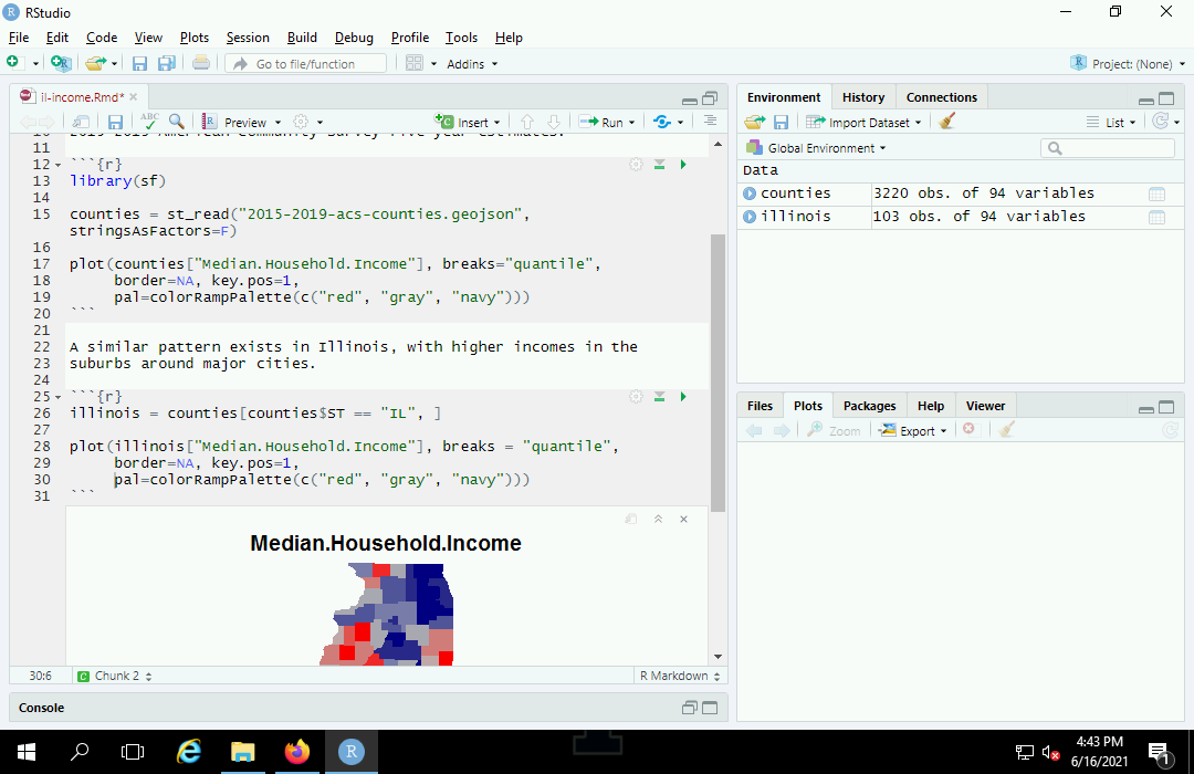
The following code subsets just counties in Illinois and then maps them.

Note that objects from previous chunks of code in the notebook persist to later chunks, and you do not need to reload the library or the counties object.

```{r}
illinois = counties[counties$ST == "IL", ]

plot(illinois["Median.Household.Income"], breaks = "quantile", 
	border=NA, key.pos=1, 
	pal=colorRampPalette(c("red", "gray", "navy")))
```

Charts

Anything that can be rendered as a visualization or text output in R can be incorporated into a notebook.

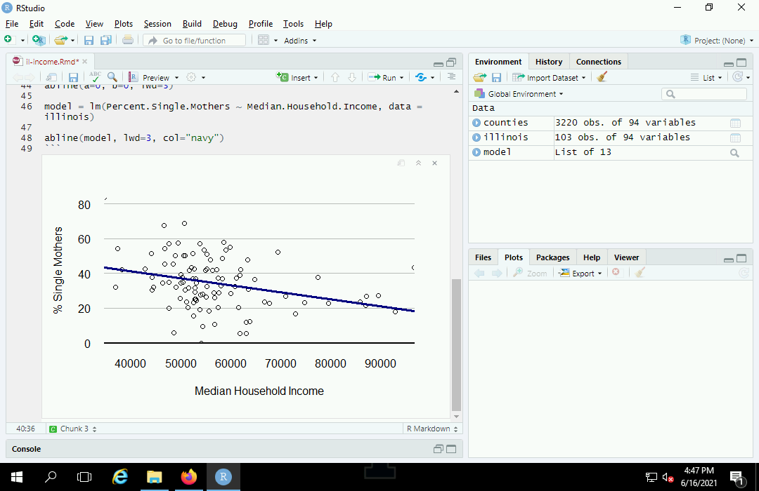
For example, this code adds an x/y scatter chart comparing median household income with the percentage of single mothers by county. It also uses the lm() creates a simple linear model in order to draw a regression line with abline() highlighting the inverse relationship between income and percent of single mothers by county.

The additional plot() formatting parameters are described in the Formatting Charts in R tutorial.

The map below shows the relationship between median household income
and the percentage of single mothers by county in Illinois.

```{r}
plot(x = illinois$Median.Household.Income, 
	y = illinois$Percent.Single.Mothers,
        las=1, fg="white", xaxs='i', yaxs='i',
        xlab="Median Household Income", ylab="% Single Mothers")

grid(nx=NA, ny=NULL, lty=1, col="#00000040")

abline(a=0, b=0, lwd=3)

model = lm(Percent.Single.Mothers ~ Median.Household.Income, data = illinois)

abline(model, lwd=3, col="navy")
```

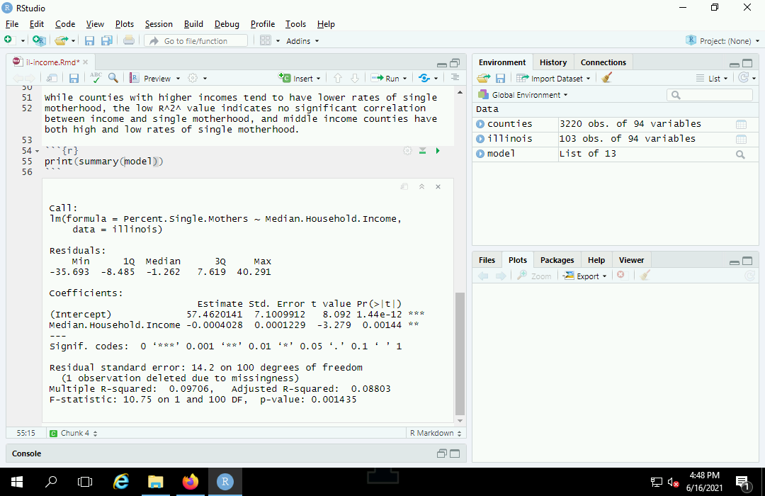
We can also add code to print() a summary() of the model showing the low R² indicating the absence of a correlation.

While counties with higher incomes tend to have lower rates of single
motherhood, the low R^2^ value indicates no significant correlation between
income and single motherhood, and middle income counties have both high and low
rates of single motherhood.

```{r}
print(summary(model))
```

Complete Notebook

The following is an example that places all of the elements above in a complete notebook.

---
title: "Median Household Income in Illinois"
author: "Michael Minn"
date: "16 June 2021"
output: html_notebook
---

This document describes the distribution of median household income
around the state of Illinois based on data from the US Census Bureau's
2015-2019 American Community Survey five-year estimates.

The map below shows that median household income is unevenly distributed
across the US, with higher incomes along the coasts and lower incomes
in rural areas, notably across the Deep South.

```{r}
library(sf)

counties = st_read("2015-2019-acs-counties.geojson", stringsAsFactors = F)

plot(counties["Median.Household.Income"], breaks = "quantile", border=NA, 
	pal=colorRampPalette(c("red", "gray", "navy")))
```

A similar pattern exists in Illinois, with higher incomes in the
suburbs around major cities.

```{r}
illinois = counties[counties$ST == "IL", ]

plot(illinois["Median.Household.Income"], breaks = "quantile", border=NA, 
	pal=colorRampPalette(c("red", "gray", "navy")))
```
The map below shows the relationship between median household income
and the percentage of single mothers by county in Illinois.

```{r}
plot(x = illinois$Median.Household.Income, 
	y = illinois$Percent.Single.Mothers,
        las=1, fg="white", xaxs='i', yaxs='i',
        xlab="Median Household Income", ylab="% Single Mothers")

grid(nx=NA, ny=NULL, lty=1, col="#00000040")

abline(a=0, b=0, lwd=3)

model = lm(Percent.Single.Mothers ~ Median.Household.Income, data = illinois)

abline(model, lwd=3, col="navy")
```

While counties with higher incomes tend to have lower rates of single
motherhood, the low R^2^ value indicates no significant correlation between
income and single motherhood, and middle income counties have both high and low
rates of single motherhood.

```{r}
print(summary(model))
```

Rendering

Notebooks can be rendered to a variety of different types of files.

If you are sharing your analysis with an audience where you want to be assured that they see the formatting exactly as you intended it, you should render as a PDF (portable document format) file.
If you want to be able to cleanly copy text and visualizations into other documents, you should share as a Word document.

Rendering can be performed from RStudio with the knit utility. Click the Preview or Knit button above the markdown text and you should see options for rendering to different types of files.

The rendering process may take a few seconds. When it is complete, RStudio should open the file for you in the appropriate application.

Knit will place the rendered output file in the working directory with a name similar to the name of your .Rmd markdown file.

Rendering a notebook to PDF or Word documents

OpenBinaryFile Error

If you are using RStudio on a machine where personal files are kept on a network drive (such as SESE-GIS or UIUC AnyWare), you may get the following error when you try to knit a document.

pandoc.exe: \\: OpenBinaryFile: does not exist (No such file or directory)

This may be because knit gets confused when the configured locations (paths) to your installed libraries are specified using a network address. You can verify this by typing the .libPaths() function at the console. If you see entries with IP addresses or quadruple slashes, this is likely the problem.

> .libPaths()
[1] "\\\\192.168.100.3/DeptUsers/minn2/Documents/R/win-library/4.0"
[2] "C:/Program Files/R/R-4.0.0.0/library"

The solution is to use a letter drive rather than the network location. On SESE-GIS, the u: drive is mapped to the network drive, so setting the .libPaths() to u: may solve the problem:

> .libPaths(c("u:/Documents/R/win-library/4.0", "c:/Program Files/R/R-4.0.0/library"))