Hypothesis Tests in R
This tutorial covers basic hypothesis testing in R.
- Normality tests
- Comparing central tendencies: Tests with continuous / discrete data
- One-sample t-test: Normally-distributed sample vs. expected mean
- Two-sample t-test: Two normally-distributed samples
- Wilcoxen rank sum: Two non-normally-distributed samples
- Weighted two-sample t-test: Two continuous samples with weights
- Comparing proportions: Tests with categorical data
- Chi-squared goodness of fit test: Sampled frequencies of categorical values vs. expected frequencies
- Chi-squared independence test: Two sampled frequencies of categorical values
- Weighted chi-squared independence test: Two weighted sampled frequencies of categorical values
- Comparing multiple groups: Tests with categorical and continuous / discrete data
- Analysis of Variation (ANOVA): Normally-distributed samples in groups defined by categorical variable(s)
- Kruskal-Wallace One-Way Analysis of Variance: Nonparametric test of the significance of differences between two or more groups
Hypothesis Testing
Science is "knowledge or a system of knowledge covering general truths or the operation of general laws especially as obtained and tested through scientific method" (Merriam-Webster 2022).
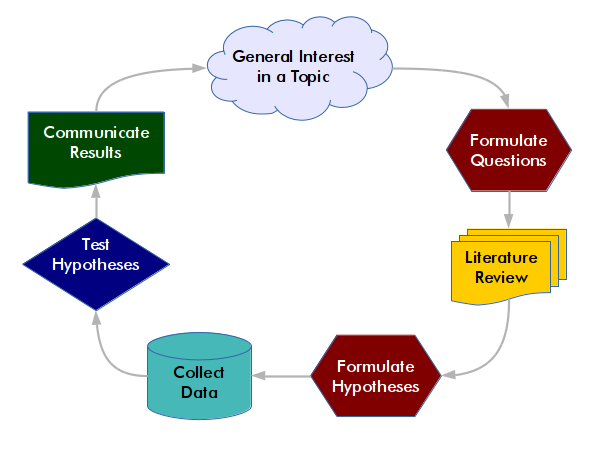
The idealized world of the scientific method is question-driven, with the collection and analysis of data determined by the formulation of research questions and the testing of hypotheses. Hypotheses are tentative assumptions about what the answers to your research questions may be.
- Formulate questions: Frame missing knowledge about a phenomenon as research question(s).
- Literature review: A literature review is an investigation of what existing research says about the phenomenon you are studying. A thorough literature review is essential to identify gaps in existing knowledge you can fill, and to avoid unnecessarily duplicating existing research.
- Formulate hypotheses: Develop possible answers to your research questions.
- Collect data: Acquire data that supports or refutes the hypothesis.
- Test hypotheses: Run tools to determine if the data corroborates the hypothesis.
- Communicate results: Share your findings with the broader community that might find them useful.
While the process of knowledge production is, in practice, often more iterative than this waterfall model, the testing of hypotheses is usually a fundamental element of scientific endeavors involving quantitative data.
The Problem of Induction
The scientific method looks to the past or present to build a model that can be used to infer what will happen in the future. General knowledge asserts that given a particular set of conditions, a particular outcome will or is likely to occur.
The problem of induction is that we cannot be 100% certain that what we are assuming is a general principle is not, in fact, specific to the particular set of conditions when we made our empirical observations. We cannot prove that that such principles will hold true under future conditions or different locations that we have not yet experienced (Vickers 2014).
The problem of induction is often associated with the 18th-century British philosopher David Hume. This problem is especially vexing in the study of human beings, where behaviors are a function of complex social interactions that vary over both space and time.

Falsification
One way of addressing the problem of induction was proposed by the 20th-century Viennese philosopher Karl Popper.
Rather than try to prove a hypothesis is true, which we cannot do because we cannot know all possible situations that will arise in the future, we should instead concentrate on falsification, where we try to find situations where a hypothesis is false. While you cannot prove your hypothesis will always be true, you only need to find one situation where the hypothesis is false to demonstrate that the hypothesis can be false (Popper 1962).
If a hypothesis is not demonstrated to be false by a particular test, we have corroborated that hypothesis. While corroboration does not "prove" anything with 100% certainty, by subjecting a hypothesis to multiple tests that fail to demonstrate that it is false, we can have increasing confidence that our hypothesis reflects reality.

Null and Alternative Hypotheses
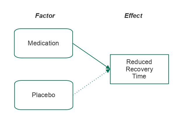
In scientific inquiry, we are often concerned with whether a factor we are considering (such as taking a specific drug) results in a specific effect (such as reduced recovery time).
To evaluate whether a factor results in an effect, we will perform an experiment and / or gather data. For example, in a clinical drug trial, half of the test subjects will be given the drug, and half will be given a placebo (something that appears to be the drug but is actually a neutral substance).
Because the data we gather will usually only be a portion (sample) of total possible people or places that could be affected (population), there is a possibility that the sample is unrepresentative of the population. We use a statistical test that considers that uncertainty when assessing whether an effect is associated with a factor.
- Statistical testing begins with an alternative hypothesis (H1) that states that the factor we are considering results in a particular effect. The alternative hypothesis is based on the research question and the type of statistical test being used.
- Because of the problem of induction, we cannot prove our alternative hypothesis. However, under the concept of falsification, we can evaluate the data to see if there is a significant probability that our data falsifies our alternative hypothesis (Wilkinson 2012).
- The null hypothesis (H0) states that the factor has no effect. The null hypothesis is the opposite of the alternative hypothesis. The null hypothesis is what we are testing when we perform a hypothesis test.
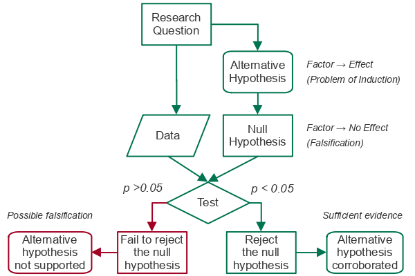
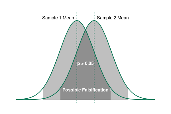
The output of a statistical test like the t-test is a p-value. A p-value is the probability that any effects we see in the sampled data are the result of random sampling error (chance).
- If a p-value is greater than the significance level (0.05 for 5% significance) we fail to reject the null hypothesis since there is a significant possibility that our results falsify our alternative hypothesis.
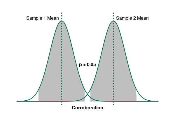
- If a p-value is lower than the significance level (0.05 for 5% significance) we reject the null hypothesis and have corroborated (provided evidence for) our alternative hypothesis.
The calculation and interpretation of the p-value goes back to the central limit theorem, which states that random sampling error has a normal distribution.
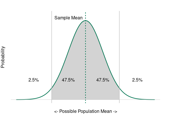
Using our example of a clinical drug trial, if the mean recovery times for the two groups are close enough together that there is a significant possibility (p > 0.05) that the recovery times are the same (falsification), we fail to reject the null hypothesis.
However, if the mean recovery times for the two groups are far enough apart that the probability they are the same is under the level of significance (p < 0.05), we reject the null hypothesis and have corroborated our alternative hypothesis.
Significance means that an effect is "probably caused by something other than mere chance" (Merriam-Webster 2022).
- The significance level (α) is the threshold for significance and, by convention, is usually 5%, 10%, or 1%, which corresponds to 95% confidence, 90% confidence, or 99% confidence, respectively.
- A factor is considered statistically significant if the probability that the effect we see in the data is a result of random sampling error (the p-value) is below the chosen significance level.
- A statistical test is used to evaluate whether a factor being considered is statistically significant (Gallo 2016).
Type I vs. Type II Errors
Although we are making a binary choice between rejecting and failing to reject the null hypothesis, because we are using sampled data, there is always the possibility that the choice we have made is an error.
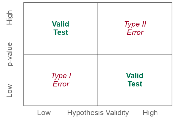
There are two types of errors that can occur in hypothesis testing.
- Type I error (false positive) occurs when a low p-value causes us to reject the null hypothesis, but the factor does not actually result in the effect.
- Type II error (false negative) occurs when a high p-value causes us to fail to reject the null hypothesis, but the factor does actually result in the effect.
The numbering of the errors reflects the predisposition of the scientific method to be fundamentally skeptical. Accepting a fact about the world as true when it is not true is considered worse than rejecting a fact about the world that actually is true.
Statistical Significance vs. Importance
When we fail to reject the null hypothesis, we have found information that is commonly called statistically significant. But there are multiple challenges with this terminology.
First, statistical significance is distinct from importance (NIST 2012). For example, if sampled data reveals a statistically significant difference in cancer rates, that does not mean that the increased risk is important enough to justify expensive mitigation measures. All statistical results require critical interpretation within the context of the phenomenon being observed. People with different values and incentives can have different interpretations of whether statistically significant results are important.
Second, the use of 95% probability for defining confidence intervals is an arbitrary convention. This creates a good vs. bad binary that suggests a "finality and certitude that are rarely justified." Alternative approaches like Beyesian statistics that express results as probabilities can offer more nuanced ways of dealing with complexity and uncertainty (Clayton 2022).
Science vs. Non-science
Not all ideas can be falsified, and Popper uses the distinction between falsifiable and non-falsifiable ideas to make a distinction between science and non-science. In order for an idea to be science it must be an idea that can be demonstrated to be false.
While Popper asserts there is still value in ideas that are not falsifiable, such ideas are not science in his conception of what science is. Such non-science ideas often involve questions of subjective values or unseen forces that are complex, amorphous, or difficult to objectively observe.
| Falsifiable (Science) |
Non-Falsifiable (Non-Science) |
|---|---|
| Murder death rates by firearms tend to be higher in countries with higher gun ownership rates | Murder is wrong |
| Marijuana users may be more likely than nonusers to misuse prescription opioids and develop prescription opioid use disorder | The benefits of marijuana outweigh the risks |
| Job candidates who meaningfully research the companies they are interviewing with have higher success rates | Prayer improves success in job interviews |
Example Data
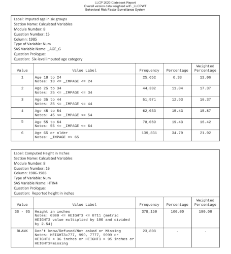
As example data, this tutorial will use a table of anonymized individual responses from the CDC's Behavioral Risk Factor Surveillance System. The BRFSS is a "system of health-related telephone surveys that collect state data about U.S. residents regarding their health-related risk behaviors, chronic health conditions, and use of preventive services" (CDC 2019).
Import
A CSV file with the selected variables used in this tutorial is available here and can be imported into R with read.csv().
responses = read.csv("2020-brfss-survey-responses.csv", as.is=T)
Guidance on how to download and process this data directly from the CDC website is available here...
Variable Types
The publicly-available BRFSS data contains a wide variety of discrete, ordinal, and categorical variables. Variables often contain special codes for non-responsiveness or missing (NA) values. Examples of how to clean these variables are given here...
The BRFSS has a codebook that gives the survey questions associated with each variable, and the way that responses are encoded in the variable values.
Normality Tests
Tests are commonly divided into two groups depending on whether they are built on the assumption that the continuous variable has a normal distribution.
- Parametric tests presume a normal distribution.
- Non-parametric tests can work with normal and non-normal distributions.
The distinction between parametric and non-parametric techniques is especially important when working with small numbers of samples (less than 40 or so) from a larger population.
The normality tests given below do not work with large numbers of values, but with many statistical techniques, violations of normality assumptions do not cause major problems when large sample sizes are used. (Ghasemi and Sahediasi 2012).
The Shapiro-Wilk Normality Test
- Data: A continuous or discrete sampled variable
- R Function: shapiro.test()
- Null hypothesis (H0): The population distribution from which the sample is drawn is not normal
- History: Samuel Sanford Shapiro and Martin Wilk (1965)
This is an example with random values from a normal distribution.
x = rnorm(30)

shapiro.test(x)
        Shapiro-Wilk normality test

data:  x
W = 0.98185, p-value = 0.8722
This is an example with random values from a uniform (non-normal) distribution.
y = runif(30)

shapiro.test(y)
        Shapiro-Wilk normality test

data:  y
W = 0.9032, p-value = 0.01007
The Kolmogorov-Smirnov Test
The Kolmogorov-Smirnov is a more-generalized test than the Shapiro-Wilks test that can be used to test whether a sample is drawn from any type of distribution.
- Data: A continuous or discrete sampled variable and a reference probability distribution
- R Function: ks.test()
- Null hypothesis (H0): The population distribution from which the sample is drawn does not match the reference distribution
- History: Andrey Kolmogorov (1933) and Nikolai Smirnov (1948)
x = rnorm(30)

ks.test(x, pnorm)
        One-sample Kolmogorov-Smirnov test

data:  x
D = 0.14587, p-value = 0.5001
alternative hypothesis: two-sided
This is an example with random values from a uniform (non-normal) distribution.
y = runif(30)

ks.test(y, pnorm)
        One-sample Kolmogorov-Smirnov test

data:  y
D = 0.54413, p-value = 7.47e-09
alternative hypothesis: two-sided
Comparing Two Central Tendencies: Tests with Continuous / Discrete Data
One Sample T-Test (Two-Sided)
The one-sample t-test tests the significance of the difference between the mean of a sample and an expected mean.
- Data: A continuous or discrete sampled variable and a single expected mean (μ)
- Parametric (normal distributions)
- R Function: t.test()
- Null hypothesis (H0): The means of the sampled distribution matches the expected mean.
- History: William Sealy Gosset (1908)
T-tests should only be used when the population is at least 20 times larger than its respective sample. If the sample size is too large, the low p-value makes the insignificant look significant..
For example, we test a hypothesis that the mean weight in IL in 2020 is different than the 2005 continental mean weight.
Walpole et al. (2012) estimated that the average adult weight in North America in 2005 was 178 pounds. We could presume that Illinois is a comparatively normal North American state that would follow the trend of both increased age and increased weight (CDC 2021).
weight.illinois = responses[responses$WEIGHT2 %in% 50:776,]

weight.illinois = weight.illinois[weight.illinois$ST %in% "IL",]

plot(density(weight.illinois$WEIGHT2), col="navy", lwd=3)

abline(v = 178, col="red", lwd=3)
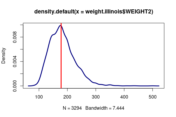
The low p-value leads us to reject the null hypothesis and corroborate our alternative hypothesis that mean weight changed between 2005 and 2020 in Illinois.
weight.test = t.test(weight.illinois$WEIGHT2, mu=178)

print(weight.test)
        One Sample t-test

data:  weight.illinois$WEIGHT2
t = 5.2059, df = 3293, p-value = 2.049e-07
alternative hypothesis: true mean is not equal to 178
95 percent confidence interval:
 180.5321 183.5918
sample estimates:
mean of x
 182.0619
One Sample T-Test (One-Sided)
Because we were expecting an increase, we can modify our hypothesis that the mean weight in 2020 is higher than the continental weight in 2005. We can perform a one-sided t-test using the alternative="greater" parameter.
The low p-value leads us to again reject the null hypothesis and corroborate our alternative hypothesis that mean weight in 2020 is higher than the continental weight in 2005.
Note that this does not clearly evaluate whether weight increased specifically in Illinois, or, if it did, whether that was caused by an aging population or decreasingly healthy diets. Hypotheses based on such questions would require more detailed analysis of individual data.
weight.test = t.test(weight.illinois$WEIGHT2, mu=178, alternative="greater")

print(weight.test)
        One Sample t-test

data:  weight.illinois$WEIGHT2
t = 5.2059, df = 3293, p-value = 1.025e-07
alternative hypothesis: true mean is greater than 178
95 percent confidence interval:
 180.7782      Inf
sample estimates:
mean of x
 182.0619
Two-Sample T-Test
When comparing means of values from two different groups in your sample, a two-sample t-test is in order.
The two-sample t-test tests the significance of the difference between the means of two different samples.
- Data:
- Two normally-distributed, continuous or discrete sampled variables, OR
- A normally-distributed continuous or sampled variable and a parallel dichotomous variable indicating what group each of the values in the first variable belong to
- Parametric (normal distributions)
- R Function: t.test()
- Null hypothesis (H0): The means of the two sampled distributions are equal.
For example, given the low incomes and delicious foods prevalent in Mississippi, we might presume that average weight in Mississippi would be higher than in Illinois.
weight = responses[responses$WEIGHT2 %in% 50:776,]

weight.illinois = weight[weight$ST %in% "IL",]

weight.mississippi = weight[weight$ST %in% "MS",]

plot(density(weight.illinois$WEIGHT2), col="navy", lwd=3)

lines(density(weight.mississippi$WEIGHT2), col="red", lwd=3)

legend("topright", legend=c("Illinois", "Mississippi"), col=c("navy", "red"), lwd=3)
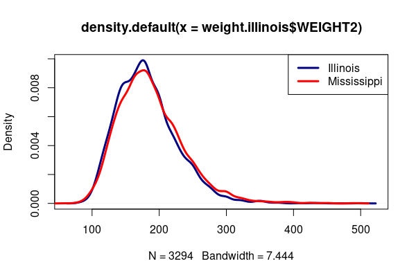
We test a hypothesis that the mean weight in IL in 2020 is less than the 2020 mean weight in Mississippi.
The low p-value leads us to reject the null hypothesis and corroborate our alternative hypothesis that mean weight in Illinois is less than in Mississippi.
While the difference in means is statistically significant, it is small (182 vs. 187), which should lead to caution in interpretation that you avoid using your analysis simply to reinforce unhelpful stigmatization.
weight.test = t.test(weight.illinois$WEIGHT2, weight.mississippi$WEIGHT2,
	alternative="less")

print(weight.test)
        Welch Two Sample t-test

data:  weight.illinois$WEIGHT2 and weight.mississippi$WEIGHT2
t = -5.5997, df = 7243.7, p-value = 1.113e-08
alternative hypothesis: true difference in means is less than 0
95 percent confidence interval:
      -Inf -3.948154
sample estimates:
mean of x mean of y
 182.0619  187.6525
Wilcoxen Rank Sum Test (Mann-Whitney U-Test)
The Wilcoxen rank sum test tests the significance of the difference between the means of two different samples. This is a non-parametric alternative to the t-test.
- Data: Two continuous sampled variables
- Non-parametric (normal or non-normal distributions)
- R Function: wilcox.test()
- Null hypothesis (H0): For randomly selected values X and Y from two populations, the probability of X being greater than Y is equal to the probability of Y being greater than X.
- History: Frank Wilcoxon (1945) and Henry Mann and Donald Whitney (1947)
The test is is implemented with the wilcox.test() function.
- When the test is performed on one sample in comparison to an expected value around which the distribution is symmetrical (μ), the test is known as a Mann-Whitney U test.
- When the test is performed to compare two samples, the test is known as a Wilcoxon rank sum test .
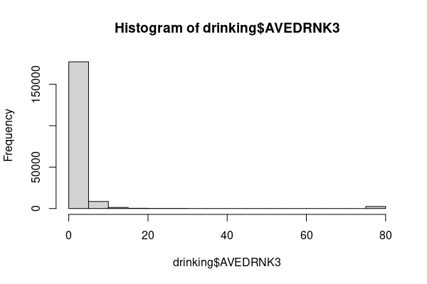
For this example, we will use AVEDRNK3: During the past 30 days, on the days when you drank, about how many drinks did you drink on the average?
- 1 - 76: Number of drinks
- 88: None
- 77: Don’t know/Not sure
- 99: Refused
- NA: Not asked or Missing
The histogram clearly shows this to be a non-normal distribution.
drinking = responses[responses$AVEDRNK3 %in% 1:88, ]

drinking$AVEDRNK3[drinking$AVEDRNK3 == 88] = 0

hist(drinking$AVEDRNK3)
Continuing the comparison of Illinois and Mississippi from above, we might presume that with all that warm weather and excellent food in Mississippi, they might be inclined to drink more. The means of average number of drinks per month seem to suggest that Mississippians do drink more than Illinoians.
drinking.illlinois = drinking[drinking$ST %in% "IL",]

drinking.mississippi = drinking[drinking$ST %in% "MS",]

print(mean(drinking.illinois$AVEDRNK3))

print(mean(drinking.mississippi$AVEDRNK3))
[1] 3.672253
[1] 5.43498
We can test use wilcox.test() to test a hypothesis that the average amount of drinking in Illinois is different than in Mississippi. Like the t-test, the alternative can be specified as two-sided or one-sided, and for this example we will test whether the sampled Illinois value is indeed less than the Mississippi value.
The low p-value leads us to reject the null hypothesis and corroborates our hypothesis that average drinking is lower in Illinois than in Mississippi. As before, this tells us nothing about why this is the case.
drinking.test = wilcox.test(drinking.il$AVEDRNK3, drinking.ms$AVEDRNK3,
	alternative="less")

print(drinking.test)
        Wilcoxon rank sum test with continuity correction

data:  drinking.il$AVEDRNK3 and drinking.ms$AVEDRNK3
W = 1515949, p-value = 0.00262
alternative hypothesis: true location shift is less than 0
Weighted Two-Sample T-Test
The downloadable BRFSS data is raw, anonymized survey data that is biased by uneven geographic coverage of survey administration (noncoverage) and lack of responsiveness from some segments of the population (nonresponse). The X_LLCPWT field (landline, cellphone weighting) is a weighting factor added by the CDC that can be assigned to each response to compensate for these biases.
The wtd.t.test() function from the weights library has a weights parameter that can be used to include a weighting factor as part of the t-test.
library(weights)

drinking = responses[responses$AVEDRNK3 %in% 1:88, ]

drinking$AVEDRNK3[drinking$AVEDRNK3 == 88] = 0

drinking.illlinois = drinking[drinking$ST %in% "IL",]

drinking.mississippi = drinking[drinking$ST %in% "MS",]

drinking.test = wtd.t.test(x = drinking.illinois$AVEDRNK3,
	y = drinking.mississippi$AVEDRNK3,
	weight=drinking.illinois$X_LLCPWT,
	weighty = drinking.mississippi$X_LLCPWT)

print(drinking.test)
[1] "Two Sample Weighted T-Test (Welch)"

$coefficients
      t.value            df       p.value
-5.637736e+00  3.430205e+03  1.862277e-08

$additional
Difference     Mean.x     Mean.y   Std. Err
-2.5176334  3.8457353  6.3633687  0.4465682
Comparing Proportions: Tests with Categorical Data
Chi-Squared Goodness of Fit
- Tests the significance of the difference between sampled frequencies of different values and expected frequencies of those values
- Data: A categorical sampled variable and a table of expected frequencies for each of the categories
- R Function: chisq.test()
- Null hypothesis (H0): The relative proportions of categories in one variable are different from the expected proportions
- History: Karl Pearson (1900)
For example, we test a hypothesis that smoking rates changed between 2000 and 2020.
In 2000, the estimated rate of adult smoking in Illinois was 22.3% (Illinois Department of Public Health 2004).
The variable we will use is SMOKDAY2: Do you now smoke cigarettes every day, some days, or not at all?
- 1: Current smoker - now smokes every day
- 2: Current smoker - now smokes some days
- 3: Not at all
- 7: Don't know
- 9: Refused
- NA: Not asked or missing - NA is used for people who have never smoked
We subset only yes/no responses in Illinois and convert into a dummy variable (yes = 1, no = 0).
smoking = responses

smoking$SMOKDAY2 = ifelse(smoking$SMOKDAY2 %in% 1:2, 1, 0)

smoking.illinois = table(smoking[smoking$ST %in% "IL", "SMOKDAY2"])

print(smoking.illinois * 100 / sum(smoking.illinois))
       0        1
88.50014 11.49986
The listing of the table as percentages indicates that smoking rates were halved between 2000 and 2020, but since this is sampled data, we need to run a chi-squared test to make sure the difference can't be explained by the randomness of sampling.
In this case, the very low p-value leads us to reject the null hypothesis and corroborates the alternative hypothesis that smoking rates changed between 2000 and 2020.
smoking.test = chisq.test(smoking.illinois, p=c(0.777, 0.223))

print(smoking.test)
        Chi-squared test for given probabilities

data:  smoking.illinois
X-squared = 248.2, df = 1, p-value < 2.2e-16
Chi-Squared Contingency Analysis / Test of Independence
- Tests the significance of the difference between frequencies between two different groups
- Data: Two categorical sampled variables
- R Function: chisq.test()
- Null hypothesis (H0): The relative proportions of one variable are independent of the second variable.
- History: Karl Pearson (1900)
We can also compare categorical proportions between two sets of sampled categorical variables.
The chi-squared test can is used to determine if two categorical variables are independent. What is passed as the parameter is a contingency table created with the table() function that cross-classifies the number of rows that are in the categories specified by the two categorical variables.
The null hypothesis with this test is that the two categories are independent. The alternative hypothesis is that there is some dependency between the two categories.
For this example, we can compare the three categories of smokers (daily = 1, occasionally = 2, never = 3) across the two categories of states (Illinois and Mississippi).
smoking = responses[responses$SMOKDAY2 %in% c(1,2,3,NA),]

smoking$SMOKDAY2[is.na(smoking$SMOKDAY2)] = 3

smoking.table = table(smoking[smoking$ST %in% c("IL", "MS"), c("ST", "SMOKDAY2")])

print(smoking.table)

plot(smoking.table)
    SMOKDAY2
ST      1    2    3
  IL  326   98 3255
  MS  720  303 5456
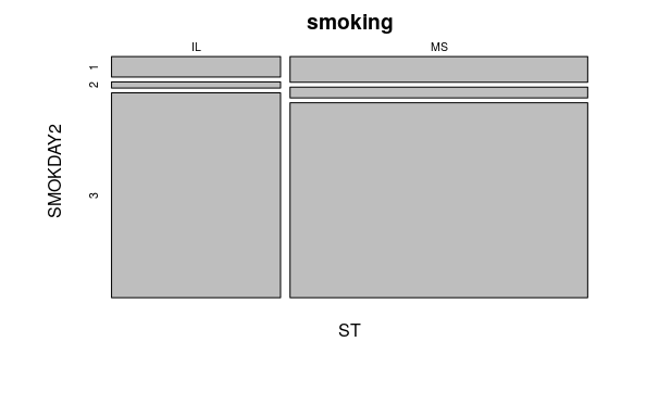
The low p-value leads us to reject the null hypotheses that the categories are independent and corroborates our hypotheses that smoking behaviors in the two states are indeed different.
smoking.test = chisq.test(smoking.table)

print(smoking.test)
        Pearson's Chi-squared test

data:  smoking
X-squared = 40.615, df = 2, p-value = 1.516e-09
Weighted Chi-Squared Contingency Analysis
As with the weighted t-test above, the weights library contains the wtd.chi.sq() function for incorporating weighting into chi-squared contingency analysis.
As above, the even lower p-value leads us to again reject the null hypothesis that smoking behaviors are independent in the two states.
library(weights)

smoking = responses[responses$SMOKDAY2 %in% c(1,2,3,NA),]

smoking$SMOKDAY2[is.na(smoking$SMOKDAY2)] = 3

smoking = smoking[smoking$ST %in% c("IL", "MS"),]

smoking.test = wtd.chi.sq(var1 = smoking$ST, var2 = smoking$SMOKDAY2,
	weight = smoking$X_LLCPWT)

print(smoking.test)
       Chisq           df      p.value
7.938529e+01 2.000000e+00 5.777015e-18
Comparing Categorical and Continuous Variables
Analysis of Variation (ANOVA)
Analysis of Variance (ANOVA) is a test that you can use when you have a categorical variable and a continuous variable. It is a test that considers variability between means for different categories as well as the variability of observations within groups.
- Data: One or more categorical (independent) variables and one continuous (dependent) sampled variable
- Parametric (normal distributions)
- R Function: aov()
- Null hypothesis (H0): There is no difference in means of the groups defined by each level of the categorical (independent) variable
- History: Ronald Fisher (1921)
As an example, we look at the continuous weight variable (WEIGHT2) split into groups by the eight income categories in INCOME2: Is your annual household income from all sources?
- 1: Less than $10,000
- 2: $10,000 to less than $15,000
- 3: $15,000 to less than $20,000
- 4: $20,000 to less than $25,000
- 5: $25,000 to less than $35,000
- 6: $35,000 to less than $50,000
- 7: $50,000 to less than $75,000)
- 8: $75,000 or more
- 77: Don’t know/Not sure
- 99: Refused
- NA: Not asked or Missing
The barplot() of means does show variation among groups, although there is no clear linear relationship between income and weight.
weight.illinois = responses[(responses$WEIGHT2 %in% 50:776) &
		(responses$INCOME2 %in% 1:8) &
		(responses$ST %in% "IL"),]

weight.list = aggregate(weight.illinois$WEIGHT2, by=list(weight.illinois$INCOME2), FUN=mean)

x = barplot(weight.list$x, names.arg=weight.list$Group.1, las=1)

text(x, 20, round(weight.list$x), cex=0.8)
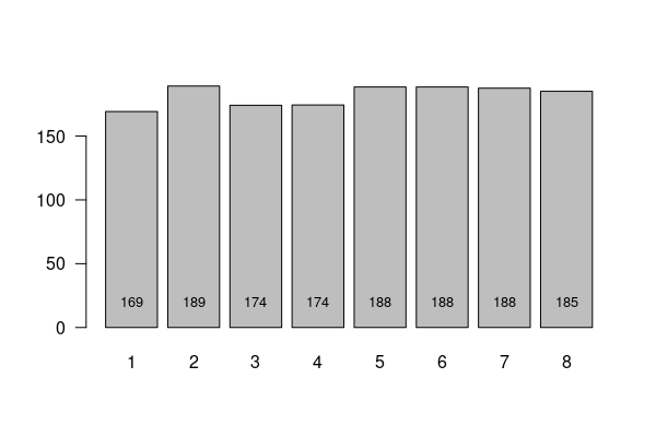
To test whether this variation could be explained by randomness in the sample, we run the ANOVA test.
The low p-value leads us to reject the null hypothesis that there is no difference in the means of the different groups, and corroborates the alternative hypothesis that mean weights differ based on income group.
However, it gives us no clear model for describing that relationship and offers no insights into why income would affect weight, especially in such a nonlinear manner.
model = aov(WEIGHT2 ~ INCOME2, data = weight.illinois)

summary(model)
              Df  Sum Sq Mean Sq F value   Pr(>F)
INCOME2        1   22301   22301   11.19 0.000836 ***
Residuals   2458 4900246    1994
---
Signif. codes:  0 ‘***’ 0.001 ‘**’ 0.01 ‘*’ 0.05 ‘.’ 0.1 ‘ ’ 1
Kruskal-Wallace One-Way Analysis of Variance
A somewhat simpler test is the Kruskal-Wallace test which is a nonparametric analogue to ANOVA for testing the significance of differences between two or more groups.
- Data: One or more categorical (independent) variables and one continuous (dependent) sampled variable
- Non-parametric (normal or non-normal distributions)
- R Function: kruskal.test()
- Null hypothesis (H0): The samples come from the same distribution.
- History: William Kruskal and W. Allen Wallis (1952)
For this example, we will investigate whether mean weight varies between the three major US urban states: New York, Illinois, and California.
weight.urban = responses[(responses$WEIGHT2 %in% 50:776) &
		(responses$ST %in% c("NY","IL","CA")),]

boxplot(WEIGHT2 ~ ST, data = weight.urban)
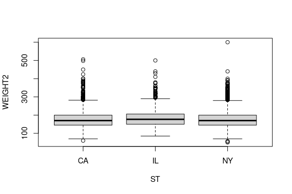
To test whether this variation could be explained by randomness in the sample, we run the Kruskal-Wallace test.
The low p-value leads us to reject the null hypothesis that the samples come from the same distribution. This corroborates the alternative hypothesis that mean weights differ based on state.
model = kruskal.test(WEIGHT2 ~ ST, data = weight.urban)

print(model)
        Kruskal-Wallis rank sum test

data:  WEIGHT2 by ST
Kruskal-Wallis chi-squared = 68.676, df = 2, p-value = 1.222e-15