Accessing Geospatial Data in Python

A vast array of geospatial data is available on the web, most notably from open data portals provided by agencies at all levels of government.

While many organizations provide their data as services or in geospatial file formats that are simple to import into Python, much of the available data is in quirky formats that can sometimes require significant time for exploration and / or cleaning before you can use the data in Python.

This tutorial will cover techniques for accessing geospatial data in Python sourced from data files and online sources.

Open vs. Proprietary Data
ArcGIS Hub

ArcGIS Hub Feature Services
ArcGIS Hub GeoJSON Files
ArcGIS Hub Shapefiles

Socrata

Socrata GeoJSON Files
Socrata CSV FIles
Socrata WKT Files

The World Bank
US Census Bureau
CSV Point Files
Tab-Delimited Files (CDC Wonder)
Excel Spreadsheets (Statistical Review of World Energy)
HTML Tables (Widipedia)
OpenStreetMap
Exporting GeoJSON
Sharing with GitHub

Open vs. Proprietary Data

Open data is "data that can be freely used, re-used and redistributed by anyone - subject only, at most, to the requirement to attribute and sharealike" (Open Knowledge Foundation 2018). Open data is free in two different ways:

Free as in beer: You do not pay anything to use it.
Free as in speech: You can use that data in any way you want.

A fundamental value of open data is interoperability, which is "the ability of diverse systems and organizations to work together" and intermix different datasets (Open Knowledge Foundation 2018).

When people can work together with a minimum of restrictions, this results greater individual productivity that, ideally, benefits society as a whole.
Governments that make their data openly available are more transparent and, ideally, more accountable to the people they govern.

The concept of open is often contrasted with proprietary. Proprietary data is data where access is controlled, usually to subscribers who pay to license use of that data.

Proprietary data can be free (as in beer) but will probably not be free (as in speech).
Free (as in beer) proprietary data is sometimes subject to license restrictions (often loosely enforced) on how the data can be used and / or redistributed.

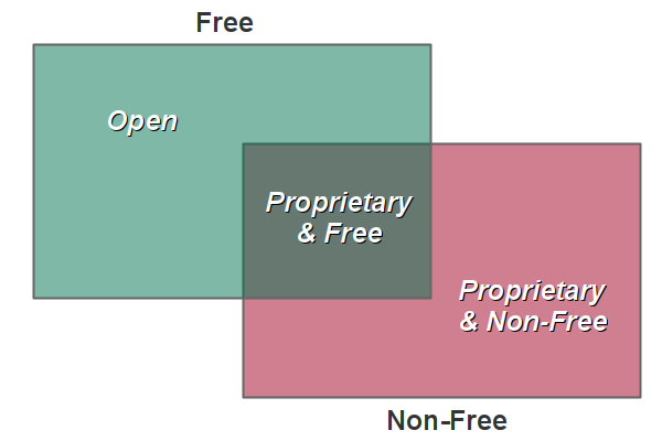
All data requires effort (and, therefore, money) to capture and maintain. So while data may be available to you at no direct cost, there are still costs associated with free data. Ultimately somebody has to pay to create, maintain and distribute that data.

In the proprietary model, the users of data users pay the costs for data, plus a profit to the company controlling the data.
In the open model, the cost is paid for by the public as a whole (such as with taxpayer-supported government data), and / or by individual companies that build business models that leverage open data with their own contributions (such as with OpenStreetMap).

Despite the ideal of perfectly interoperable systems built on open data, the current reality is that free and open geospatial data is commonly made available across a variety of different types of website in a variety of different formats.

ArcGIS Hub

Open data portals often use content management systems (CMS) to organize and provide access to their different data sets.

ArcGIS Hub is a CMS for geospatial data which was created by ESRI (the dominant company in enterprise GIS) and is tightly integrated with their ArcGIS Online and ArcGIS Server software.

Some cities that use ArcGIS Hub for their open geospatial data include:

ArcGIS Hub Feature Services

ArcGIS Hub makes geospatial data available as feature services.

Feature services are streams of vector data (points, lines, and polygons) that can be accessed by GIS software directly through application programmer interfaces (APIs).

APIs implement service access with REST endpoints, which are named based on the type of communications protocol they use (representational state transfer).

A REST endpoint is a URL to a service on the server that includes subfolders and parameters needed to identify a specific service. For example, this is the REST endpoint URL to the US Energy Information Administrations's power plant locations feature service.

https://services7.arcgis.com/FGr1D95XCGALKXqM/arcgis/rest/services/Power_Plants_Testing/FeatureServer/0/query?outFields=*&where=1%3D1&f=geojson")

GeoJSON is a contemporary open geospatial data format based on the web data format JSON (JavaScript object notation) that was finalized in 2008. When you have the option to access GeoJSON through a feature service or downloadable file, that will probably be your safest option for getting readable data.

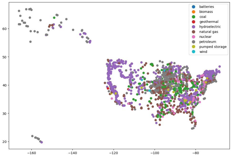
The following video demonstrates how to get a REST endpoint for a feature service of power plants from the US Energy Information Administration's U.S. Energy Atlas implemented with ArcGIS Hub.

Find the data set you want to use (Power Plants).
Select I want to use this.
Under API copy the GeoJSON link.
Use that link to load the data with geopandas.read_file()

Getting REST endpoint URL from ArcGIS Hub

import geopandas

import matplotlib.pyplot as plt

power_plants = geopandas.read_file("https://services7.arcgis.com/FGr1D95XCGALKXqM/arcgis/rest/services/Power_Plants_Testing/FeatureServer/0/query?outFields=*&where=1%3D1&f=geojson")

power_plants.plot("PrimSource", legend=True)

plt.show()

A map of US power plants created with a GeoJSON feature service from ArcGIS Hub

ArcGIS Hub GeoJSON Files

GeoJSON data can also be downloaded as a file that you can keep on local storage.

A GeoJSON file may be preferred over a feature service when you need a snapshot of the data at a specific point in time since feature services can be updated at any time.
A GeoJSON file may be preferred over a feature service when you need reliable access since feature services are dependent on the provider and can disappear at any time.
A GeoJSON file may be preferred over a feature service because feature services are often not designed for high volumes of mission-critical activity, so they can be slow and give unreliable performance.

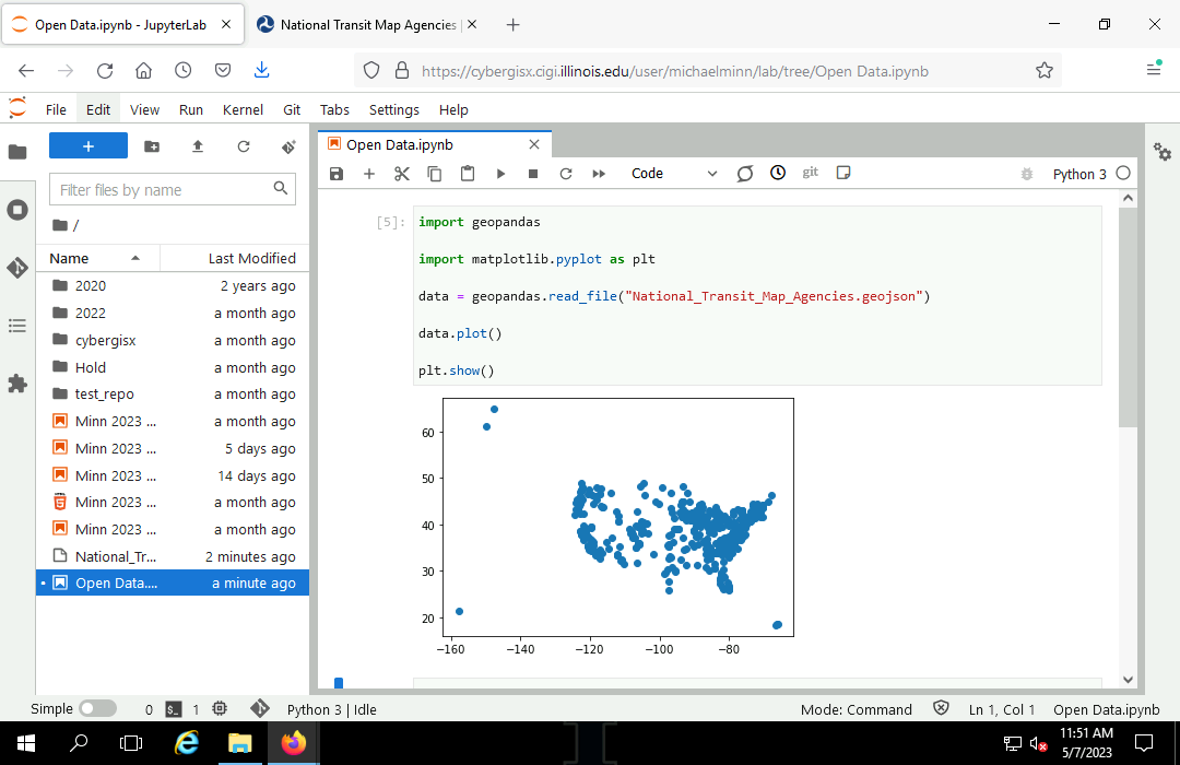
The following example shows how to download a GeoJSON file of transit agency headquarters from the US Bureau of Transportation Statistics National Transportation Atlas Database and open it in a Jupyter notebook.

Find the data set you want to use (National Transit Map Agencies).
Select Download.
Download the GeoJSON file.
Upload the file to the system where your notebook is running.
Load the file with geopandas.read_file()

Downloading a GeoJSON file from ArcGIS Hub

import geopandas

import matplotlib.pyplot as plt

transit_agencies = geopandas.read_file("2023-transit-stops.geojson")

transit_agencies.plot(markersize = 4)

plt.show()

A map of US transit agency headquarters created with GeoJSON file from ArcGIS Hub

ArcGIS Hub Shapefiles

GeoJSON files open erratically on ESRI software (ArcGIS Pro and ArcGIS Online), so if you will be sharing data with ESRI users, you may want to download your data as a shapefile.

The shapefile is a geospatial data file format developed by ESRI in the late 1990s that that is supported by a wide variety of software from other vendors, and as such has become, probably, the most common format for distributing geospatial data through open data portals.

While the age of the shapefile format is reflected in its numerous limitations (most notably a column name length limit of 10 characters), this format is supported by a wide variety of GIS software and is a safe format that is still commonly used for distributing open geospatial data by government agencies.

The term shapefile is a misnomer since a shapefile is actually a collection of at least three (and usually more) separate files that store the locational data, the characteristics associated with those locations, and other information about the data. When copying a shapefile, it is critical that you include all of these different files, or the file will either not open or be missing important components.

Some common files associated with a shapefile include (listed by the file extension):

.shp: Contains the feature geometry (points, lines, polygons)
.shx: An index file that indicates where specific features are in the .shp file
.dbf: A dBase IV database file of attributes associated with each of the shapes in the .shp file
.prj: The coordinate system and projection used by the feature geometry (optional)
.cpg: The character encoding used by the attributes (optional)
.qpj: The coordinate system and projection in a format used by QGIS (optional)

For convenience, the separate files in a shapefile are usually compressed into a single .zip archive file for distribution on websites and servers.

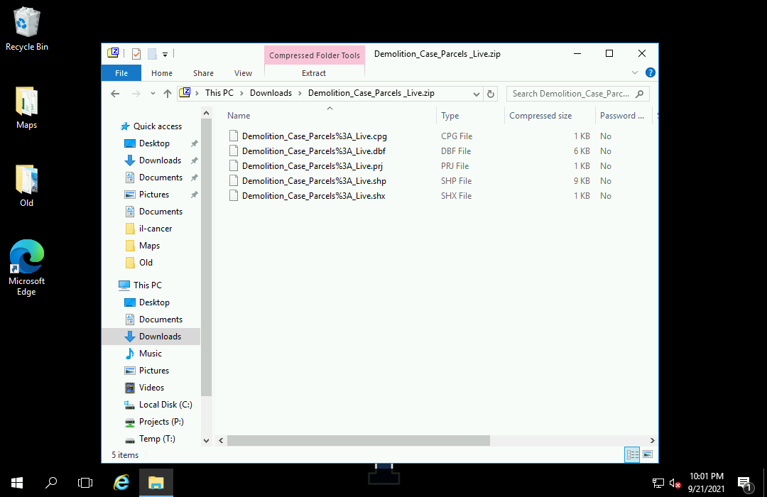
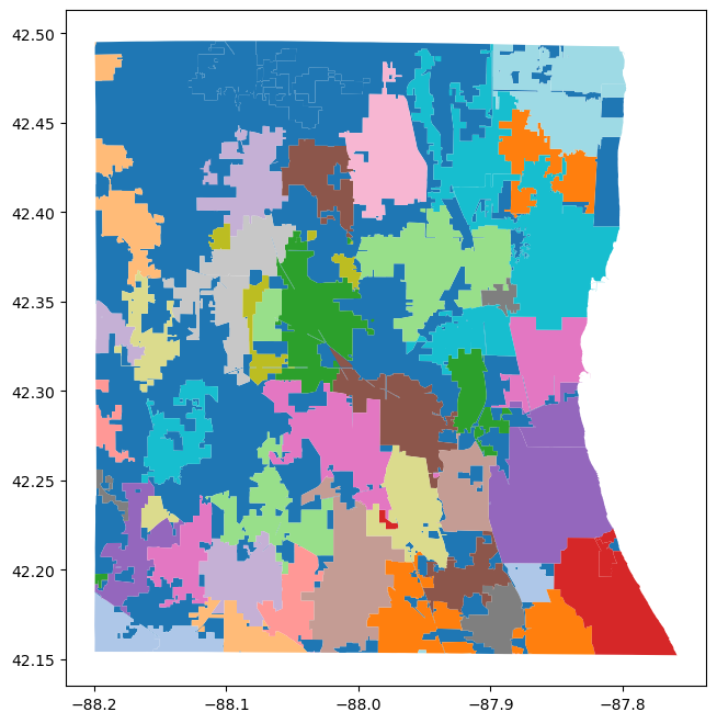
Multiple physical files associated with a single shapefile

The following example shows how to download a zipped shapefile of the 56 (!) separate municipalities in Lake County, IL from the Lake County, IL Open Data & Records Hub and open it in Jupyter Hub.

Find the data set you want to use (Municipal Boundaries).
Select Download.
Download the zipped Shapefile.
Upload the zip file to your notebook environment or a public server like GitHub.
Load the zip file with geopandas.read_file()

Downloading a shapefile from ArcGIS Hub

import geopandas

import matplotlib.pyplot as plt

municipalities = geopandas.read_file("2023-lake-county-municipalities.zip")

municipalities.plot(cmap="tab20")

plt.show()

A map of municipalities in Lake County, IL created from a shapefile from ArcGIS Hub

Socrata

A common open source CMS used by government agencies for disseminating geospatial and non-geospatial data is Socrata.

Socrata is a general purpose CMS rather than a CMS specifically designed for distributing geospatial data for web maps like ArcGIS Hub. However, for use with Python, Socrata provides geospatial data access that is on par with ArcGIS Hub.

Some cities that use Socrata for their open geospatial data include:

Socrata GeoJSON Data

The Chicago Open Data Portal uses the Socrata CMS, and geospatial data sets usually have an export option for GeoJSON.

The links to GeoJSON exports can be used to download GeoJSON files, or can be used directly in the GeoPandas read_file() function to access the data directly from the Socrata servers.

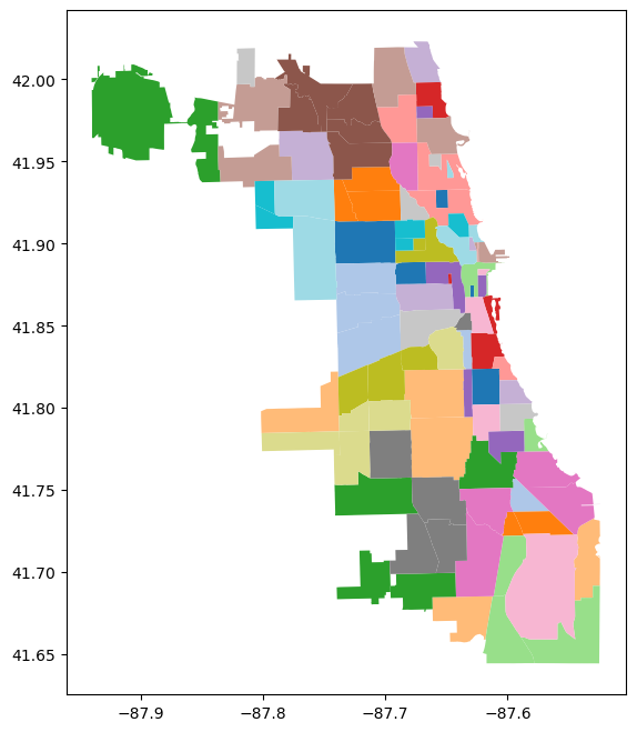
The following video demonstrates how to access a GeoJSON file of Chicago neighborhoods.

Find the data set you want to use (Boundaries - Neighborhoods).
Select Export.
Copy the GeoJSON link.
Use that link to load the data with geopandas.read_file()

Accessing GeoJSON data directly from a Socrata website

import geopandas

import matplotlib.pyplot as plt

neighborhoods = geopandas.read_file("https://data.cityofchicago.org/api/geospatial/bbvz-uum9?method=export&format=GeoJSON")

neighborhoods.plot(cmap="tab20")

plt.show()

neighborhoods.columns

A map of neighborhoods in Chicago using GeoJSON data from Socrata

Socrata CSV Files

The comma-separated variable (CSV) format is a text format that arranges data in rows, with column cells separated by commas. CSV files can be thought of as spreadsheets, and they are commonly edited using spreadsheet software like Microsoft Excel, but CSV files do not preserve formatting information.

CSV files can be used for geospatial data with columns of latitude and longitude associated on each row with specific attributes at those latitudes and longitudes. Most CSV files can only represent points, so for lines (like roads) and areas (like neighborhoods or census tracts) you need to save data in a specialized geospatial data file format like the shapefile.

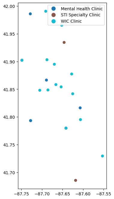
Point data in data portals like Socrata is sometimes made available as tables with latitudes and longitudes rather than in geospatial data formats like shapefiles.

Find the data set you want to use (Chicago Department of Public Health Clinic Locations).
Select Export.
Copy the CSV link.
Use that link to load the data into a DataFrame with pandas.read_csv()
Use geopandas.points_from_xy() to convert the lat/long to a GeometryArray.
Use geopandas.GeoDataFrame() to combine the geometries and the attributes from the CSV into a GeoDataFrame that can be plotted.

Importing lat/long points downloaded from a Socrata data portal

import pandas

import geopandas

csv = pandas.read_csv("https://data.cityofchicago.org/api/views/kcki-hnch/rows.csv?accessType=DOWNLOAD")

points = geopandas.points_from_xy(csv["Longitude"], csv["Latitude"])

clinics = geopandas.GeoDataFrame(csv, geometry = points, crs="EPSG:4326")

subplot = clinics.plot("Clinic Type", legend=True)

plt.show()

clinics.columns

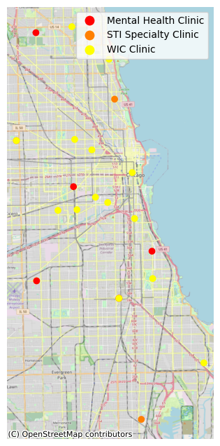
A map of CDPH clinics in Chicago using lat/long CSV data from Socrata

Points need some kind of geographic context to be meaningful. This example uses contextily to add a base map to a plot.

import contextily as cx

csv = pandas.read_csv("https://data.cityofchicago.org/api/views/kcki-hnch/rows.csv?accessType=DOWNLOAD")

points = geopandas.points_from_xy(csv["Longitude"], csv["Latitude"])

clinics = geopandas.GeoDataFrame(csv, geometry = points, crs="EPSG:4326")

clinics = clinics.to_crs("EPSG:3857") # Web Mercator

subplot = clinics.plot("Clinic Type", legend=True, cmap="autumn")

cx.add_basemap(subplot, source=cx.providers.OpenStreetMap.Mapnik)

subplot.set_axis_off()

plt.show()

A map of CDPH clinics in Chicago with a base map

Socrata WKT CSV Files

You may occasionally find a CSV file from Socrata that contains a column with geometries represented as well-known text (WKT) that contain geometry type names followed by a list of coordinates.

This example is the cooling centers list from the City of Chicago Open Data portal. The WKT column is named LOCATION.

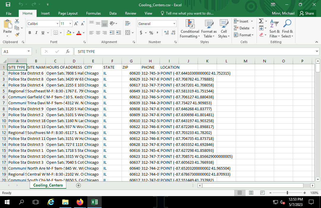
WKT can be converted to geometries using the geopandas.GeoSeries.from_wkt() function.

The drop.na() method call to remove rows with blank locations is critical or your from_wkt() call will fail with the cryptic error message "TypeError: Expected bytes, got float."

import pandas

import geopandas

import matplotlib.pyplot as plt

csv = pandas.read_csv("https://data.cityofchicago.org/api/views/msrk-w9ih/rows.csv?accessType=DOWNLOAD")

csv = csv.dropna(subset="LOCATION")

points = geopandas.GeoSeries.from_wkt(csv["LOCATION"])

centers = geopandas.GeoDataFrame(csv, geometry = points, crs="EPSG:4326")

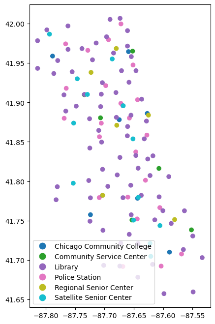
centers.plot("SITE TYPE", legend=True)

plt.show()

centers.info()

A map of summer cooling centers in Chicago using WKT in CSV data from Socrata

The World Bank

The World Bank is a group of international agencies that provide funding and knowledge to promote economic development in developing countries. The World Bank is one of the Bretton Woods institutions founded as part of an international agreement made during a 1944 conference in Bretton Woods, NH that was convened to plan for reconstruction after World War II and promote international cooperation that would help avoid World War III.

The World Bank collects a vast array of country-level data (including public health data), and makes it available to the general public on their data.worldbank.org data portal as part of their mission to be a source of knowledge that promotes economic development.

See this tutorial on Geospatial Data from the World Bank for details on how to access World Bank data in Python using precompiled GeoJSON, downloadable tables, or the World Bank API.

US Census Bureau

The US Census Bureau (USCB) is the part of the US federal government responsible for collecting data about people and the economy in the United States. The Census Bureau has its roots in Article I, section 2 of the US Constitution, which mandates an enumeration of the entire US population every ten years (the decennial census) in order to set the number of members from each state in the House of Representatives and Electoral College (USCB 2017). The Census Act of 1840 established a central office for conducting the decennial census, and that office became the Census Bureau under the Department of Commerce and Labor in 1903 (USCB 2021).

See this tutorial on Geospatial Data from the US Census Bureau for details on how to access USCB data from Python using precompiled GeoJSON, downloaded tables, or through the Census Bureau API.

CSV Point Files

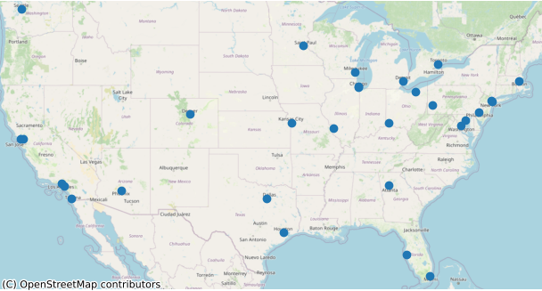
Points can also be loaded from CSV files using the GeoPandas points_from_xy function if you are working with data files that have columns of latitude and longitude.

Point maps usually need some kind of base map to provide geographic context. Contextily can be used to display tiled base maps using the add_basemap function, although Contextily base maps can be slow to load, and highly-detailed base maps can make it difficult to distinguish point symbology.

import pandas
import geopandas
import contextily
import matplotlib.pyplot as plt

csv = pandas.read_csv('https://michaelminn.net/tutorials/data/2019-mlb-ballparks.csv')

points = geopandas.points_from_xy(csv['Longitude'], csv['Latitude'])

ballparks = geopandas.GeoDataFrame(csv, geometry = points, crs='EPSG:4326')

ballparks = ballparks.to_crs("EPSG:3857")

axis = ballparks.plot()

contextily.add_basemap(axis, source = contextily.providers.OpenStreetMap.Mapnik)

axis.set_axis_off()

plt.show()

A map of US major league baseball parks from a CSV file with latitudes and longitudes

Tab-Delimited Files (CDC Wonder)

Tab-delimited files are similar to comma-separated variable (CSV) files except tab characters are used instead of commas to separate fields on each row. Use of tabs causes fewer problems when the data contains commas or quotation marks.

If you discover that downloaded table data is coming in as one big column with no column names, you may have a tab-delimited file rather than a CSV file.

Tab-delimited files can be read using the Pandas read_table() function.

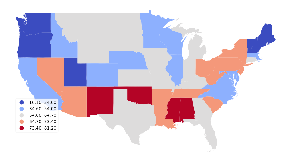
The example below shows how to download COVID deaths by state from the US Centers for Disease Control and Prevention (CDC) WONDER online database.

Go to wonder.cdc.gov
Select Underlying cause of death
Select 2018-2021: Underlying Cause of Death by Single-Race Categories

Agree to the usage terms on the About page.
1. Organize table layout: Group Results By State
6. Select cause of death: Search for COVID (code U07.1)
Select Export Results
Send request to the database.

In Windows Explorer, rename the file to something short but meaningful (2021-covid-deaths.txt).
Upload the file to your notebook environment or a shared server.
Add the file path as a parameter to pandas.read_table().
geopandas.read_file() the appropriate TIGER shapefile area polygons.
merge() the polygons with the table data.
plot() or analyze as needed.

Loading a tab-delimited file from CDC WONDER

import pandas

import geopandas

import matplotlib.pyplot as plt

covid = pandas.read_table("2021-covid-deaths.txt")

states = geopandas.read_file("https://www2.census.gov/geo/tiger/GENZ2022/shp/cb_2022_us_state_5m.zip")

states = states.to_crs("EPSG:3857")

states = states[~states["STUSPS"].isin(['AK', 'HI', 'PR'])]

states = states.merge(covid, left_on="name", right_on="Geographic Area Name (NAME)")

subplot = states.plot("", scheme="naturalbreaks", cmap="coolwarm", 
	legend=True, legend_kwds={"bbox_to_anchor":(0.2, 0.4)})

subplot.set_axis_off()

plt.show()

An import of tab-delimited CDC WONDER data of COVID death rates by state

Excel Spreadsheets (Statistical Review of World Energy)

Data provided as Excel spreadsheets (.xlsx or .xls) is commonly formatted for printing, and will often need to be cleaned and exported to a CSV file for input into Python.

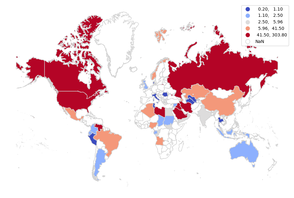
For this example we use petroleum reserves by country (Oil - Proved Reserves) from the data tables .xlsx file for the Energy Institute's Statistical Review of World Energy (formerly the bp Statistical Review of World Energy).

Remove all unneeded columns, leaving only the needed data and place name columns.
Remove all informational rows above and below the data.
Remove all totals rows.
Rename the data columns in row one with short but meaningful names that will be convenient field names for your code.
Modify place names as needed to be consistent with your polygon data. For joins, place names in the table data must exactly match the place names in the polygon data. This will often need to be fixed by making an initial join and finding the countries where the data did not join. The specific locations that need to be changed will vary by data set, and with this particular table, those countries are as follows:

Equatorial Guinea (Eq. Guinea)
Republic of Congo (Congo)
Russian Federation (Russia)
South Sudan (S. Sudan)
Trinidad & Tobago (Trinidad and Tobago)
US (United States of America)

Save the worksheet to a CSV file (2022-oil-reserves.csv).
Upload the CSV file to your notebook server or a public server like GitHub.

Loading data from a .xlsx file for the Statistical Review of World Energy

import geopandas

import matplotlib.pyplot as plt

oil_reserves = pandas.read_csv("2022-oil-reserves.csv")

countries = geopandas.read_file("https://michaelminn.net/tutorials/data/2023-natural-earth-countries.geojson")

countries = countries.to_crs("EPSG:3857")

countries = countries.merge(oil_reserves, how="left", left_on="NAME", right_on="Country")

subplot = countries.plot("2020", scheme="quantiles", cmap="coolwarm", 
	edgecolor="lightgray", legend=True,
	missing_kwds={"color","white"})

subplot.set_axis_off()

plt.show()

Map of proved oil reserves in billions of barrels (Energy Institute)

HTML Tables (Wikipedia)

Data is sometimes made available on websites as HTML tables on web pages. If you have no other download options, it is possible to copy that data into CSV files for import into Python.

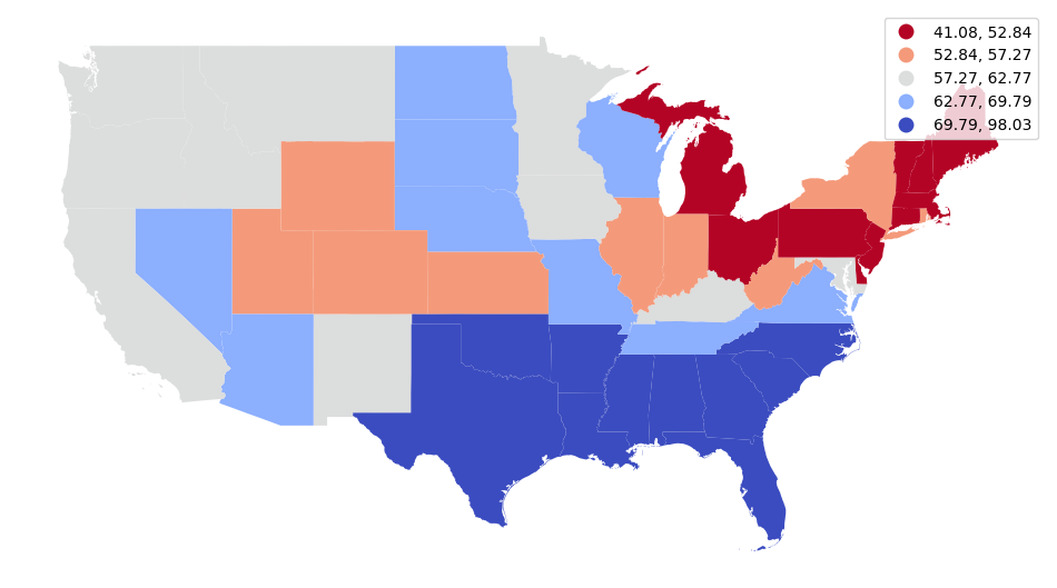
This example uses the state vote total and percent table for the 1932 US presidential election from Wikipedia.

Note that Wikipedia is an online encyclopedia and the data in Wikipedia usually comes from some other original source. Before using data copied from Wikipedia, you may want to look at the references for the original data source and use that instead so you can be assured of the most current and accurate data.

Select the data on the web page and copy it into a blank spreadsheet.
Remove all unneded rows and columns.
Modify row one as needed to be short but meaningful names for your fields.
Make sure all rows in the location column have valid location names.
Remove non-numeric characters from numeric column values.
Save As the spreadsheet as a Comma Separated Variable (CSV) file (1932-results.csv).
Upload the CSV file to your notebook server or a public server like GitHub.

Creating a feature service from an geocoded HTML table

import geopandas

import matplotlib.pyplot as plt

results = pandas.read_csv("1932-results.csv")

states = geopandas.read_file("https://www2.census.gov/geo/tiger/GENZ2022/shp/cb_2022_us_state_5m.zip")

states = states.to_crs("EPSG:3857")

states = states.merge(results, left_on="NAME", right_on="State")

subplot = states.plot("Dem_Percent", scheme="quantiles", cmap="coolwarm_r", legend=True)

subplot.set_axis_off()

plt.show()

Map of 1932 US presidential election results (Official publications from state election agencies)

OpenStreetMap

OpenStreetMap (OSM), is a collection of geospatial data built by a community of mappers that contribute and maintain data about roads, trails, cafés, railway stations, and much more, all over the world. While the main site is similar to Google Maps and OSM is often thought of as an open version of Google Maps, the primary focus of the OSM project is the collecting and dissemination of the data itself.

The project was initially started by Steve Coast in 2004 following the lead of Wikipedia as an open-source encyclopedia, and OSM is often referred to as the "Wikipedia of maps." As with open-source software, the open data model contrasts with the proprietary data model under the belief that community is stronger by standing on each other's shoulders rather than standing on each other toes.

The OSMnx package provides convenient access to OSM data as GeoDataFrames.

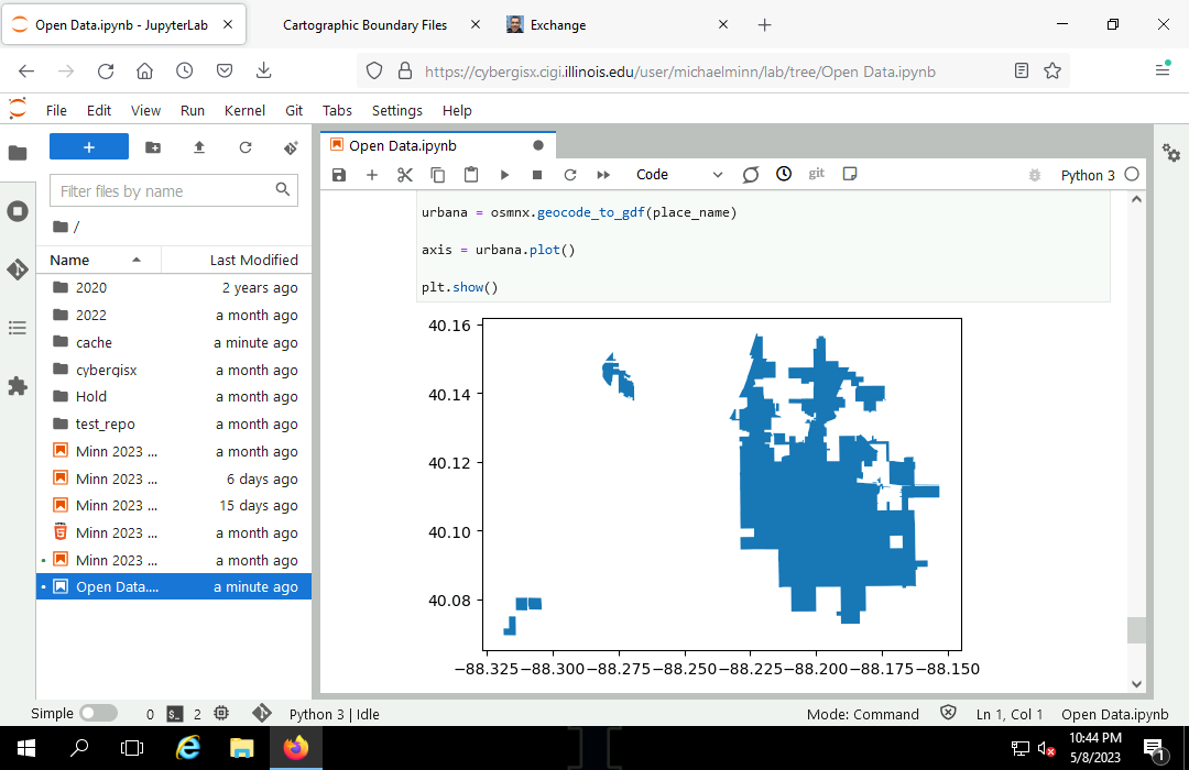
First, confirm that your search area is valid.

import osmnx

import geopandas

import matplotlib.pyplot as plt

place_name = "Urbana, IL"

urbana = osmnx.geocode_to_gdf(place_name)

subplot = urbana.plot()

plt.show()

Perform a search based on tag contents.

tags = {'amenity':'restaurant'}

restaurants = osmnx.geometries_from_place(place_name, tags)

restaurants["name"].head()

element_type  osmid     
node          287470185        Siam Terrace
              1700549689    The Red Herring
              2174331934           Po' Boys
              2180117733     Courtyard Cafe
              2180118609         Basil Thai
Name: name, dtype: object

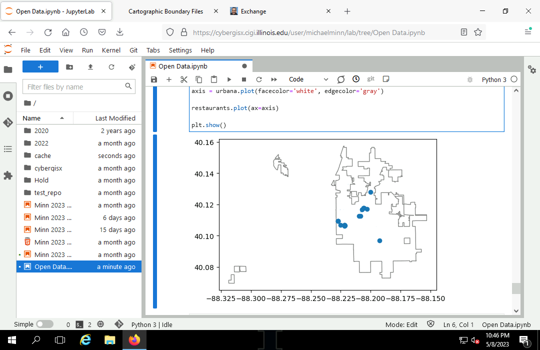
If desired, plot the returned features.

subplot = urbana.plot(facecolor='white', edgecolor='gray')

restaurants.plot(ax=subplot)

plt.show()

Restaurants in Urbana, IL from OpenStreetMap

Exporting GeoJSON

You may wish to save your GeoDataFrame to a file in cases where:

You need to preserve a snapshot of the data at a particular point in time.
The service(s) you source your data from are slow, unreliable, or unstable.
The data takes a significant amount of time to process from original sources.
You wish to make sure your collaborators are using the exact same data you are using.

The GeoPandas to_file() method can be used to write a variety of different file formats, including GeoJSON and shapefiles.

Unless you are sharing with people who will be using your data in an ESRI desktop environment (ArcGIS Pro), the open GeoJSON format will likely be your safest choice for maintaining your data in a format that will preserve unadulterated contents and be readable in the near future.
To assure there is no confusion regarding your projection you should use the GeoPandas to_crs() method to assure the data is in WGS 1984 lat/long.
This example uses the restaurants data set created above.

restaurants.to_crs("EPSG:4326").to_file('2023-urbana-restaurants.geojson', driver='GeoJSON')

Sharing with GitHub

If you will be exchanging your Python code with a collaborator or instructor, it may be of value for you to place your data files on a server so your code will be portable without the difficulty of having to also exchange your data files.

GitHub is "an Internet hosting service for software development and version control using Git" (Wikipedia 2023).

GitHub provides a wide variety of features for synchronizing development environments that can become quite complex. However, some simple features can be useful for basic sharing of files.

If you have a data file that you wish to share so people who have your notebook can access that data through the internet, you can upload it to GitHub and get a shared link to incorporate in your notebook.

Add file and Upload files with the data file. GitHub will create simple renderings of geospatial data files.
Copy the shared link from the Download button.
Incorporate that link in your notebook code.

Sharing a data file on GitHub