Geospatial Data from the World Bank
This tutorial covers acquisition of World Bank indicator data in ArcGIS Online, ArcGIS Pro, Python, and R.
The World Bank
The World Bank is a group of international agencies that provide funding and knowledge to promote economic development in developing countries. The World Bank is one of the Bretton Woods institutions founded as part of an international agreement made during a 1944 conference in Bretton Woods, NH that was convened to plan for reconstruction after World War II and promote international cooperation that would help avoid World War III.
Precompiled Data
If you just need commonly-used variables and are uninterested in getting data for a particular year, the easiest course of action may be to use this precompiled GeoJSON file available on this website, which is also available in ArcGIS Online as the Minn 2022 World Bank Indicators feature service.
ArcGIS Pro
Under Analysis and Tools, use the Export Features tool to copy the data from the Minn 2022 World Bank Indicators feature service into the project database.
Although you can use a feature service directly on a map in ArcGIS Pro, copying the data into a new feature class in the project database will make it faster and easier to perform analysis, and assure that the data is readily available if the original feature service is unavailable or is discontinued.
ArcGIS Online
Add the Minn 2022 World Bank Indicators feature service from ArcGIS Online as a new layer.
Python
You can read the GeoJSON file directly into a GeoDataFrame using the GeoPandas read_file() function.
import geopandas

import matplotlib.pyplot as plt

countries = geopandas.read_file("https://michaelminn.net/tutorials/data/2022-world-bank-indicators.geojson")

countries = countries.to_crs("ESRI:54030")

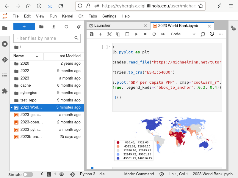
axis = countries.plot("GDP per Capita PPP", cmap="coolwarm_r", scheme="quantiles",
	legend=True, legend_kwds={"bbox_to_anchor":(0.3, 0.4)})

axis.set_axis_off()

plt.show()
R
You can read the GeoJSON file directly into an object using the sf st_read() function.
library(sf)

countries = st_read("https://michaelminn.net/tutorials/data/2022-world-bank-indicators.geojson")

countries = st_transform(countries, "ESRI:54030")

redblue = colorRampPalette(c("red", "lightgray", "navy"))

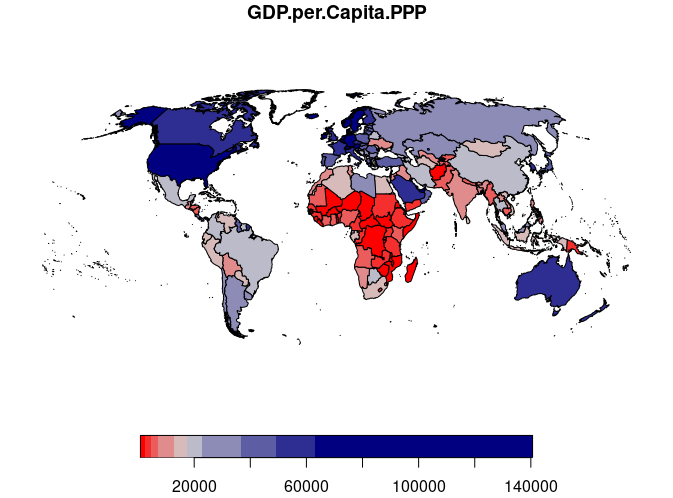
plot(countries["GDP.per.Capita.PPP"], pal=redblue, breaks="quantile")
Using World Bank Table Data
The World Bank aggregates a vast array of country-level data as indicators available as tabular data from the World Bank Open Data portal. By joining that data with country polygons, you can create choropleth maps and perform geospatial analysis.
Downloading Table Data
- Search for an indicator of interest on data.worldbank.org. The variable used in this example is infant mortality rate per 1,000 live births.
- Click the Download button and download an Excel file, which should open in a spreadsheet program on your machine.
- Go to the Data sheet and remove the unneeded rows and columns.
- The first three rows are metadata that can be removed. Make sure the top row (row #1) are meaningful names that you can use for referencing the fields.
- Remove any columns you won't need, but be sure to keep the Country Name and Country Code columns, which will be needed later.
- Make sure the columns you want to use have enough data. Some indicators have data for only a limited number of countries, and you may need to manually copy data between columns so there is data for all countries you want to analyze or visualize.
- If you want to add additional indicators, download those Excel files and copy the columns directly into your original spreadsheet. Excel files for different indicators have the same number of rows in the same order.
- Save As the file as a Comma-separated variable (CSV) file under a meaningful name.
Mapping World Bank Table Data in ArcGIS Pro
In order to create a choropleth map from a table of data that contains only names of locations, you need to perform an attribute join that associates rows of table data with polygon features in a feature class that indicate where to draw that data on the map.
A join is a database operation where two tables are connected based on common key values.
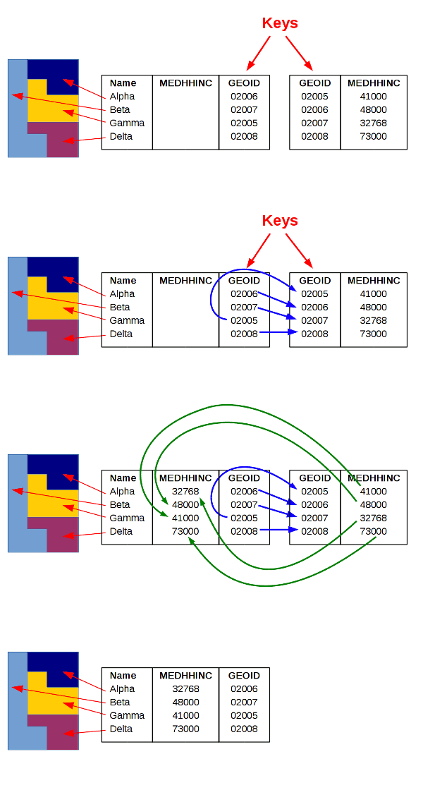
In this example, we join a data table with polygon features using a key of standard (ISO) country codes.
- Download and process the table data as described above.
- Under Analyze and Tools, search for the Export Features tool to bring the country polygons into the project geodatabase.
- Input Table: The table of country polygons (Minn 2023 World Polygons feature service)
- Output Feature Class: Provide a meaningful name (Infant_Mortality)
- Under Analyze and Tools, search for the Join Field tool.
- Input Table: The table of country polygons you imported above.
- Input Join Field: ISO_A3
- In Join Table, navigate to the spreadsheet you edited.
- The Join Table Field should be the three-letter ISO Country Code that is a field common to both the table data and the GeoJSON file. Standardized ISO country codes are better join keys than country names because variations in spelling of country names can cause some features to fail to be joined (e.g. Iran vs. Islamic Republic of Iran).
- Run the tool and you should have new fields on the polygon feature class in your project geodatabase.
Mapping World Bank Table Data in ArcGIS Online
- Download and process the table data as described above.
- Store the table data:
- On your ArcGIS Online Content page, click New Item.
- Browse Your Device to find the CSV file on your local machine.
- On the How would you like to add this file? screen, select Add...and create a hosted feature layer or table.
- On the Fields screen, verify that all fields are appropriate types. Make sure all numbers have a type Double (double precision floating point).
- On the Location settings screen, select None since you will be joining this with polygons.
- Give the new layer a meaningful name unique to your organization (Minn 2022 Infant Mortality).
- When the service information page pops up, Open in Map Viewer.
- Under Analysis and Tools, select Join Features to join the table with polygons:
- Target Layer: Browse ArcGIS Online and use the Minn 2023 World Polygons layer.
- Join Layer: Use the table you uploaded to ArcGIS Online.
- Target Field: The country codes (ISO_A3)
- Join Field: The Country Code in the table.
- Output Name: Provide a meaningful name (Minn 2023 Infant Mortality).
- The join may take a minute or two.
- Communicate: Create the map.
- Change the styling if desired and Save Layer so that styling is the default when the layer is loaded in the future.
- Save the map under a meaningful name. Using the same name as the feature service will aid in remembering the two items are connected (Minn 2023 Infant Mortality)
- Adjust Share map as needed (Everyone).
- Copy the URL from the location bar to share the map.
Mapping World Bank Table Data in Python
- Download and clean up the table data as described above.
- Pandas is a Python package working with tabular data.
- GeoPandas is a Python package for working with geospatial data.
- Matplotlib is a Python package for plotting graphs.
- CSV files can be read into Pandas DataFrames using the read_csv() function.
- Find the URL to the appropriate TIGER cartographic boundary zipped shapefile from the link on the page shown above.
- Read the cartographic boundary file directly from the USCB website into a GeoDataFrame object using the read_file() function.
- Use the to_crs() method to reproject the data to the North America Lambert Conformal Conic projection suitable for North America (ESRI 102009).
- Join the table DataFrame with the county polygon GeoDataFrame using the Pandas merge() method and the GEO_ID fields in the two objects.
- To map only the continental 48 states, we exclude Alaska, Hawaii, and Puerto Rico using their FIPS codes.
import pandas

import geopandas

import matplotlib.pyplot as plt

table_data = pandas.read_csv("infant_mortality.csv")

countries = geopandas.read_file("https://michaelminn.net/tutorials/data/2023-natural-earth-countries.geojson")

countries = countries.to_crs("ESRI:54030")

countries = countries.merge(table_data, left_on="ISO_A3", right_on="Country Code")

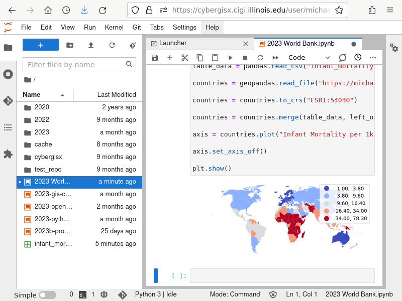
axis = countries.plot("Infant Mortality per 1k", cmap="coolwarm", legend=True, scheme="quantiles")

axis.set_axis_off()

plt.show()
Mapping World Bank Table Data in R
- Download and clean up the table data as described above.
- Read the table data into an R data.frame using the read.csv() function.
- Load the country polygons into a simple features data.frame using st_read().
- Reproject the polygons into a cartographically appropriate projection with st_transform(). For this data we use the North America Lambert Conformal Conic projection suitable for North America (ESRI 102009).
- merge() the polygons and the table on the ISO country code fields.
- Create an appropriate diverging colorRampPalette.
- plot() a choropleth colored by the desired variable.
library(sf)

table_data = read.csv("infant_mortality.csv")

countries = st_read("https://michaelminn.net/tutorials/data/2023-natural-earth-countries.geojson")

countries = st_transform(countries, "ESRI:54030")

countries = merge(countries, table_data, by.x="ISO_A3", by.y="Country.Code")

redblue = colorRampPalette(c("navy", "lightgray", "red"))

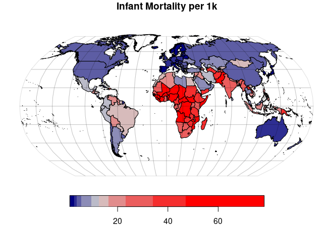
plot(countries["Infant.Mortality.per.1k"], pal=redblue, breaks="quantile")
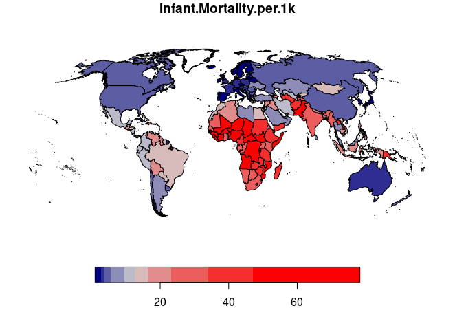
If you want to save a copy of your processed data for later use, you can use the st_write() function to create a variety of different types of geospatial data files.
st_write(counties, "2022-infant-mortality.geojson")
Using the World Bank Data API
The World Bank provides an application programmers interface (API) that can be used for directly accessing indicator data. The API provides a variety of options for selecting data (example calls).
for this example, we will use the call that gets indicator data for the most recent year for all available countries in the following form:For example, to get the most recent available years for the Mortality rate, infant (per 1,000 live births), the API URL would be:
http://api.worldbank.org/v2/country/all/indicator/SP.DYN.IMRT.IN?mrnev=1&per_page=300
- SP.DYN.IMRT.IN is the World Bank name for the infant mortality indicator. Acquisition of other indicator names is described below.
- mrnev=1 indicates to get data for the most recent year. Many indicators do not have data for all years. This should be used with caution if you need data for specific years or want to be assured of that you are using current data.
- per_page=300 indicates that the GET should acquire up to 300 rows. This will cover all available countries.
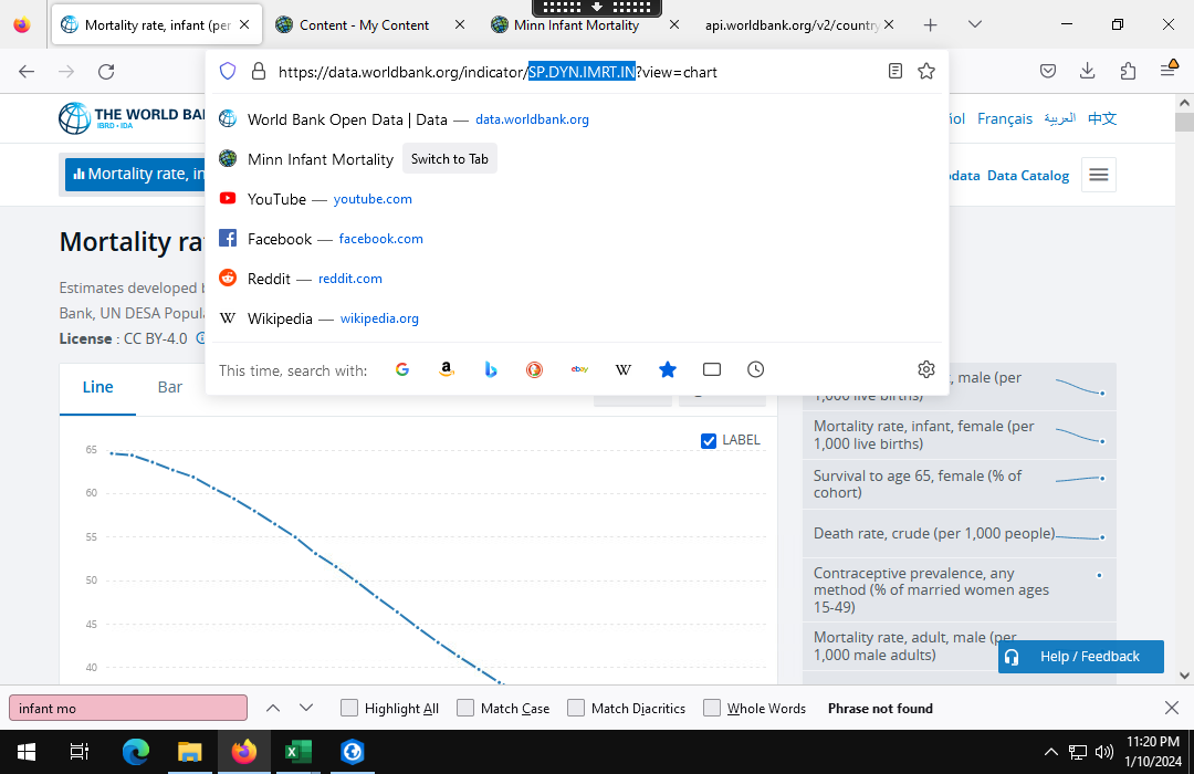
To find the desired indicator ID, find the indicator page in data.worldbank.org and view the indicator ID in the page URL.
Mapping World Bank API Data in Python
The only geospatial components the World Bank tables contain are country names and ISO country codes, so to map the data you will need to perform an attribute join to connect the data to polygons that can be used for mapping.
A join is a common database operation where two data sets are connected to form a single data set. An attribute join connects two datasets based on common key values.

The pandas.read_xml() function can be used to load the XML data from the API in Python.
You can remove and rename columns to make the data more usable, especially if you wish to add additional indicators.
Use ISO_A3 for the ISO country code to make the merge() easier below.
Use the GeoPandas merge() method to join the table data using the ISO codes from a GeoJSON file of Natural Earth country polygons.
import pandas
import geopandas
import matplotlib.pyplot as plt

table_data = pandas.read_xml("https://api.worldbank.org/v2/country/all/indicator/SP.DYN.IMRT.IN?mrnev=1&per_page=300")

table_data = table_data[["countryiso3code", "value"]]

table_data = table_data.rename(columns = {"countryiso3code":"ISO_A3", "value":"Infant Mortality per 1k"})

countries = geopandas.read_file("https://michaelminn.net/tutorials/data/2023-natural-earth-countries.geojson")

countries = countries.merge(table_data, on="ISO_A3")

countries = countries.to_crs("EPSG:3857")

axis = countries.plot("Infant Mortality per 1k", scheme="quantiles", cmap="coolwarm",
	legend=True, legend_kwds={"bbox_to_anchor":(0.3, 0.4)})

axis.set_axis_off()

plt.show()
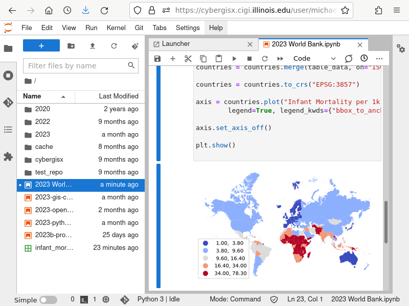
Additional indicators can be added by repeating the read_xml, rename, and merge steps.
table_data = pandas.read_xml("https://api.worldbank.org/v2/country/all/indicator/NY.GDP.PCAP.PP.CD?mrnev=1&per_page=300")

table_data = table_data[["countryiso3code", "value"]]

table_data = table_data.rename(columns = {"countryiso3code":"ISO_A3", "value":"GDP Per Capita"})

countries = countries.merge(table_data, on="ISO_A3")

print(countries.info())
RangeIndex: 193 entries, 0 to 192
Data columns (total 6 columns):
 #   Column                       Non-Null Count  Dtype
---  ------                       --------------  -----
 0   NAME                         193 non-null    object
 1   FORMAL_EN                    192 non-null    object
 2   ISO_A3                       193 non-null    object
 3   geometry                     193 non-null    geometry
 4   Infant Mortality per 1k      193 non-null    float64
 5   GDP Per Capita               193 non-null    float64
dtypes: float64(2), geometry(1), object(3)
memory usage: 9.2+ KB
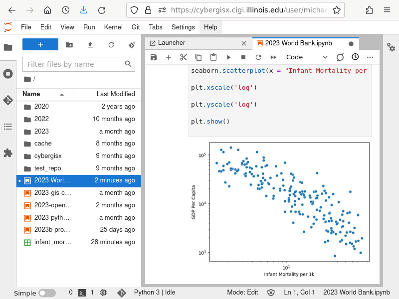
Combining indicators can be especially useful for performing correlation and regression analysis.
import seaborn

seaborn.scatterplot(x = "Infant Mortality per 1k", y = "GDP Per Capita", data=countries)

plt.xscale('log')

plt.yscale('log')

plt.show()
Mapping World Bank API Data in R
The only geospatial components the World Bank tables contain are country names and ISO country codes, so to map the data you will need to perform an attribute join to connect the data to polygons that can be used for mapping.
A join is a common database operation where two data sets are connected to form a single data set. An attribute join connects two datasets based on common key values.

We join the table data using the ISO codes from a GeoJSON file of Natural Earth country polygons using the sf merge() function.
library(sf)
library(XML)
library(xml2)

table_data = read_xml("https://api.worldbank.org/v2/country/all/indicator/SP.DYN.IMRT.IN?mrnev=1&per_page=300")

table_data = xmlParse(table_data)

table_data = xmlToDataFrame(table_data)

table_data = table_data[,c("countryiso3code","date","value")]

table_data$value = as.numeric(table_data$value)

names(table_data) = c("ISO_A3", "Year", "Infant Mortality per 1k")

countries = st_read("https://michaelminn.net/tutorials/data/2023-natural-earth-countries.geojson")

countries = st_transform(countries, "ESRI:54030")

countries = merge(countries, table_data, all.x=T)

redblue = colorRampPalette(c("navy", "lightgray", "red"))

plot(countries["Infant Mortality per 1k"], pal=redblue, breaks="quantile", reset=F)

graticule = st_read("https://michaelminn.net/tutorials/data/2023-graticule.geojson")

graticule = st_transform(graticule, st_crs(countries))

plot(graticule$geometry, col=NA, border="#00000020", add=T)
