Geospatial Data from the US Census Bureau
Revised 4 June 2026
This tutorial covers basic techniques for acquiring and joining US Census Bureau (USCB) data. While focusing on ArcGIS Pro, this tutorial also includes information on using USCB data in the ArcGIS Online Map Viewer, Python, and R.
- US Census Bureau Data
- US Census Bureau Downloads and Joins
- USCB Table Data
- TIGER Shapefiles
- FIPS Codes
- GEOIDs
- Joining USCB Table Data to Polygons
- Joining Non-USCB Data on FIPS Codes
- Joining Non-USCB Data on County Names
- Symbolizing Change
- TIGER Infrastructure Shapefiles
- Project Geodatabase
- USCB Data from Secondary Sources
- Feature Services
- ArcGIS Online Feature Services
- Counties Filtered by State
- County Tracts Filtered by GEOID
- Living Atlas Features
- Public Feature Services
- ArcGIS Online
- Python
- R
- USCB API

All videos in this tutorial are silent.
US Census Bureau Data
The US Census Bureau (USCB) is the part of the US federal government responsible for collecting data about people (demographics) and the economy in the United States. The Census Bureau has its roots in Article I, section 2 of the US Constitution, which mandates an enumeration of the entire US population every ten years (the decennial census) in order to set the number of members from each state in the House of Representatives (the lower house of the US Congress) and Electoral College (that selects the US President) (USCB 2017). The Census Act of 1840 established a central office for conducting the decennial census, and that office became the Census Bureau under the Department of Commerce and Labor in 1903 (USCB 2021).
The American Community Survey
Among the Census Bureau's many programs is the American Community Survey (ACS), an ongoing survey that provides information on an annual basis about people in the United States beyond the basic information collected in the decennial census. The ACS is commonly used by a wide variety of researchers when they need information about the general public.
Unlike the constitutionally-mandated decennial census which is only taken every ten years, the ACS continuously surveys people in America's communities so that the ACS data can be more detailed and current than the decennial census. However, because the ACS is a survey rather than a complete count like the decennial census, there is uncertainty about how accurately the sampling represents the facts on the ground, and that uncertainty is expressed in a statistical margin of error (MOE) on most ACS values (US Census Bureau 2018).
Spatial Aggregation
In order to preserve the confidentiality of respondents (and the associated willingness of people to respond to highly-personal questions), the US Census Bureau generally only releases data that has been aggregated (combined) into areas at various geographic scales:
- National data represents the United States as a whole.
- States are the fifty governmental jurisdictions into which the United States is divided. Non-state territories like Guam and Puerto Rico are also generally included in state-level data.
- Counties are the largest territorial divisions for local governments within the fifty states of the United States.
- Core-Based Statistical Areas (CBSA) represent metropolitan areas based around central (core) cities that are connected by social and economic ties. CBSAs can cross county and state lines.
- Places are incorporated cities and unincorporated communities. Each place is contained within one state, although place boundaries can cross county lines.
- ZIP Codes Tabulation Areas (ZCTA) are simplifications of the ZIP code delivery service areas used by the US Post Office. ZCTAs often cross social boundaries (like neighborhoods), so they are often problematic for social research.
- Census tracts are subdivisions of counties that are drawn based on clearly identifiable features to ideally contain around 4,000 residents, although in practice the range of population is usually between 1,200 and 8,000 (USCB 2019).
- Block groups are subdivisions of some census tracts. Block group data is unreliable for social analysis due to random noise added for disclosure avoidance.

Temporal Aggregation
Although ACS data is captured through surveys that are administered on an ongoing basis, it is aggregated into time-periods to improve geographic coverage and reduce margin of error.
ACS data is released annually in aggregation by two different time-periods.
| One-Year Estimates | Five-Year Estimates |
|---|---|
| Useful when you need the most current data about an characteristic that changes frequently | Useful when you need the most accurate data about a characteristic that stays fairly stable over time |
| Useful for areas that are changing rapidly | Useful for areas that are well-established |
| Often has gaps in sparsely-populated rural areas | Data is more complete |
| Based on fewer surveys, so it has wider margins of error | Based on more surveys, so it has lower margins of error |
Community Profile Pages
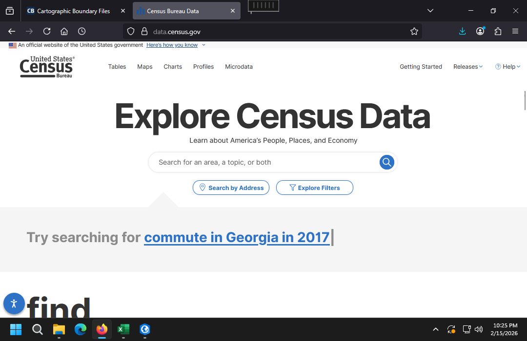
If you are looking for quick information on a specific state, county, city or community, the USCB provides profile pages in data.census.gov that include basic demographic information about population, income, education, etc.
You can access a profile page by typing the name of the area of interest into the search bar and waiting for it to autocomplete. If there is a profile page, a link to that page will appear for you to select.
US Census Bureau Downloads
The US Census Bureau makes their data available as downloadable tables from https://data.census.gov. There is a vast amount of open data available, but the volume of that data and the cumbersome design of the website require quite a bit of effort to make it usable in GIS software.
USCB Table Data
Data from a variety of different USCB programs is available on data.census.gov for download as table data.
These ACS demographic profile (DP) tables contain useful groups of data:
- DP02 Selected Social Characteristics (marriage, fertility, education, ancestry)
- DP03 Selected Economic Characteristics (employment, sectors, income)
- DP04 Selected Housing Characteristics (housing size, age, and costs)
- DP05 Demographic and Housing Estimates (race, ethnicity, and age groups)
The video below demonstrates downloading a variable for percent of homes with electric heat from the DP04 table with county-level data from data.census.gov.
- From the data.census.gov home page, search for the desired table (DP04). The default table shows values for the entire USA.
- Click the vintage selector under the table heading to select the specific data release. This example uses 2019-2023 five-year estimates.
- Click Geos to select the type of geographic area. For this example, we will use County and All counties in Illinois.
- Click Download Table.
- Download the zipped CSV.
- In the Windows File Explorer, Extract All files from the .zip archive.
- Open the file with a name containing the word "data" in it.
- Remove all columns except the GEO_ID (needed to join to the area polygons later) and the data column(s) (Percent_Electric_Heat DP04_0065PE). Be aware that values are often available for total counts and percentages.
- Remove the 2nd row with the descriptive column information and make sure the top header row has meaningful name(s).
- Look through the rows and remove any rows with non-numeric data.
- Save as the spreadsheet as a CSV file under a meaningful name (Electric_Heat.csv).
TIGER Shapefiles
While the data downloaded from data.census.gov only contains place names and GEO_IDs, the US Census Bureau makes polygons available that can be joined to USCB table data for spatial analysis and mapping.
The Topologically Integrated Geographic Encoding and Referencing (TIGER) database is a collection of geospatial data maintained by the US Census Bureau and made available to the public as shapefiles.
- TIGER/Line cartographic boundary files are simplified representations of selected geographic areas from the TIGER database that are specifically designed for small scale thematic mapping.
- TIGER/Line polygons can be joined to tabular census data for mapping and spatial analysis.
- The core TIGER/Line files are available, and include other geographic features useful for mapping like roads, railroads, and water features.
Shapefiles utilize a file format developed by ESRI in the 1990s that is actually a collection of files that each contain separate information, such as the coordinates, attributes, projection, and metadata.
- Because all these files need to be kept together, shapefiles are commonly distributed in .zip archives that collect and compress the separate files into a single, compact file with .zip at the end of the name.
- Despite the limitations of the shapefile format (most notably constraining field names to ten characters), the format is supported by a wide variety of software, and is still commonly used to store and distribute geospatial data.
The following video shows how to download a shapefile of county polygons and import it into a feature class project geodatabase in ArcGIS Pro.
- Go to the USCB's TIGER Cartographic Boundary Files page and download the appropriate type of geography. Use the highest resolution file unless you will be publishing a web map.
- In the Windows file explorer, Extract the shapefile contents into a folder in the Downloads folder.
- Use the
Export Features tool to copy the counties
data from the shapefile into the project geodatabase.
- Input Features: Browse to find the .shp file. You may need to click the refresh button to be able to see newly downloaded data.
- Output Feature Class: Browse to the project geodatabase and provide a name (Counties). Note that you must explicitly browse into the project geodatabase or the tool by default will simply copy the shapefile into another shapefile.
FIPS Codes
FIPS (Federal Information Processing Standards) codes are used to uniquely identify geographies in USCB data. FIPS codes for different geographies can be found with Google.
A full list of current FIPS codes for different area types is available on the US Census Bureau website.
FIPS codes build left to right from the more general to the more specific.
- State codes are two digits. For example, the FIPS code for Illinois is 17.
- County codes add three digits to the right of the state code. For example, the FIPS code for Cook County, IL is 17031.
- Census tract codes add an additional six digits to the county code. For example, the FIPS code for the census tract containing the Willis Tower (Sears Tower) in downtown Chicago, IL is 17031839100.
GEOIDs
FIPS codes are commonly used as GEO_ID values in US Census Bureau data.
Because purely numeric FIPS codes are ambiguous about exactly what type of geography they represent, US Census Bureau data often includes fully-qualified GEOIDs (GEOIDFQ) that append a prefix to a FIPS code that clearly indicates what type of area the FIPS code represents.
- The GEOIDFQ will be in a column named GEO_ID (in USCB data tables), GEOIDFQ (in TIGER shapefiles), or AFFGEOID (in older data).
- GEOIDFQs avoid the issue with leading zeroes being removed from FIPS codes when software represents the GEOIDs as numbers in spreadsheets or feature classes.
GEOIDFQ prefixes also have specific subfields:
- The first three digits specify the type of area: 040 for states, 050 for counties, 140 for census tracts, and 310 for core-based statistical areas (metropolitan areas).
- The next four digits represent the geographic variant and component, which are usually 0000 for states, counties, and tracts.
- The letters US
- The FIPS code
For example:
- 0400000US17 is the GEOID for Illinois.
- 0500000US17031 is the GEOID for Cook County, Illinois.
- 1400000US17031839100 is the GEOID for the census tract containing the Willis Tower.
- 310M500US16980 is the GEOID for the Chicago-Naperville-Elgin, IL-IN-WI CBSA (Chicago metropolitan area).
Joining USCB Table Data to Polygons
A join is a database operation where two tables are connected based on common key values.
An attribute join attaches a table of attribute data to a table of geospatial data based key field(s) common to both tables.
Attribute joins can be used to connect data from external tables (such as in a CSV file) to geospatial locations defined in feature classes that comes from USCB shapefiles or feature classes of secondary data.

To join USCB table data to USCB polygon feature class, we join on the GEO_ID field in the downloaded table data and the GEOIDFQ field in the polygon feature class.
- Open the Join Features tool.
- Target Layer: Select the polygon layer (Counties).
- Join Layer: Browse to the CSV file (Electric_Heat.csv).
- Output Dataset: Provide a meaningful name (Electric_Heat).
- Join Operation: Join one to many
- Attribute Relationship: GEOIDFQ (target field) to GEO_ID (join field)
- Symbolize the updated layer to verify the new fields have been joined into the data.
Joining Non-USCB Data on FIPS Codes
Geospatial table data from non-USCB sources occasionally includes FIPS codes for areas that can then be joined with TIGER shapefiles or secondary data GEOIDFQ for import into ArcGIS Pro.
There are multiple common challenges to joining with FIPS codes from non-USCB sources:
- FIPS codes often have leading zeros (e.g. 01 for Alabama) that will be removed by spreadsheet software, resulting in name mismatches that cause joins to fail.
- FIPS codes often import as numeric values that cannot be joined with the text codes in TIGER polygon data.
- FIPS codes are sometimes abbreviated, such as using only the three digit county FIPS code in state-provided data without the two-digit state FIPS prefix needed to join with five-digit FIPS codes in TIGER polygon data.
The solution to these problems is to convert your FIPS codes into GEOIDFQ in your spreadsheet program before importing and joining the CSV in ArcGIS Pro.
For example, the downloadable county level data for the US Religion Census from the Association of Statisticians of American Religious Bodies contains a FIPS code numeric FIPS code field.
- In a spreadsheet program, clean up the CSV and add a GEOIDFQ column.
- Use the CONCATENATE function with the county GEOIDFQ prefix (0500000US) to create a GEOIDFQ field.
- If the FIPS code is in a numeric format, use the TEXT(cell, "00000") function to convert the numeric cells into five-digit FIPS codes.
- Remove formatting so numbers do not come in as text.
- Remove extraneous non-data rows.
- Export to a CSV file with a meaningful name (2020_Religion_Census).
- Use the Export Table tool to bring the CSV file in as a table. If used directly in Join Features, some CSV file joins will fail with an Error 120036 field(s) not found in dataset error.
- Input Table: The CSV file (Religion_2020.csv)
- Output Table: Provide a meaningful name (Religion_2020)
- Use the Export Features tool to copy the counties data from the feature service.
- Input Features: Browse ArcGIS Online for the feature service (Minn 2019-2023 ACS) and select the counties layer.
- Output Feature Class: Browse to the project geodatabase and provide a name (Counties).
- Use the Join Features tool to join the CSV table to the polygons.
- Target Layer: Browse to the exported features (Counties).
- Join Layer: Browse to the data table (Religion_2020).
- Output Name: Browse to the project geodatabase and provide a meaningful name (Religion_Counties).
- Join Operation: Join one to many
- Attribute Relationship: Select the GEOIDFQ field in the polygons and the new GEOIDFQ field in the CSV table.
- Symbolize the updated layer to verify the new fields have been joined into the data.
Joining Non-USCB Data on County Names
Attribute joins can be used to join county-level table data to TIGER polygons based on county names for choropleth mapping.
Be aware that attribute joins require that the names in the two data sets match exactly, and using place names for joins can result in mismatches or a complete failure to join any features.
- TIGER/Line shapefiles provide county names in title case and you will need to preprocess your CSV file for county names if they capitalized in any other manner.
- You may also need to make iterative changes to your CSV names for spelling variations like St. (St. Louis vs. St Louis) and De (De Witt vs. DeWitt vs. Dewitt).
- If you are joining county data for multiple states, you will also need to have a common key for the state name or abbreviation because county names are not unique across the 50 US states. For example, in the US there are 31 Washington counties and 26 Jefferson counties.
- If a FIPS code is available, those will generally be more accurate than joining on county names.
This example uses county-level results in Illinois from the 1960 US presidential election from the Illinois Secretary of State via Wikipedia.
- Copy the table into a spreadsheet program.
- Remove all unnecessary columns and rows, leaving one header row.
- Where applicable, remove (find and replace) percent signs to that the software interprets the column as numeric.
- Save the data as a CSV file (IL_1960_Election.csv).
- Use Join Features tool to join the CSV table to the polygons.
- Target Layer: Select the polygon layer (Counties).
- Join Layer: Browse to the table CSV file (IL_1960_Election.csv).
- Output Name: Browse to the project geodatabase and provide a meaningful name (IL_1960_Election).
- Join Operation: Join one to many
- Attribute Relationship: Select the Name field in the features and the county name field (County) in the CSV file.
- If you see missing features (DeWitt = De Witt), fix the CSV and re-run the tool.
Symbolizing Change
TIGER Infrastructure Shapefiles
TIGER/Line shapefiles are available for a variety of geographic features. These features can be used for creating base maps.
- Go to the USCB's TIGER/Line Shapefiles page, choose the web interface, and download the desired geometries.
- Using Windows Explorer, open the file, copy the contents, and paste them into the Downloads directory.
- Bring the data into the project geodatabase with the Export Features tool.
- Input Features: Browse to the shapefile.
- Output Feature Class: Browse to the project geodatabase and provide a name (Rail_Lines). Note that you need to browse to the project geodatabase because if you just type a name in this box, the tool will just copy to another shapefile.
Project Geodatabase
When working with data from shapefiles and tables in ArcGIS Pro, the data should be saved in the project geodatabase to keep the project data together and avoid losing external files. This is why many examples in this tutorial use Export Features tool to copy the data from shapefiles or feature services into the project geodatabase.
- A geodatabase is special type of database containing "a collection of geographic datasets of various types" (ESRI 2020).
- A feature class is a geographic dataset within a geodatabase that contain features of the same geometric type (points, lines, polygons) and a common set of attributes (ESRI 2024).
- Each individual geographic entity in a feature class is called a feature. For example, in a feature class for roads in a county, each road segment would be a feature (ESRI 2020).
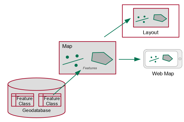
A project geodatabase is the default geodatabase used for storing feature classes that are imported or created as part of an ArcGIS Pro project.
- The project geodatabase is a file geodatabase kept in the project folder (Documents\ArcGIS\Projects\project_name) under the name project_name.gdb
- The project geodatabase does not store data brought in to maps with Add Data from feature services or from geospatial data files (like shapefiles) unless you explicitly copy that data into the project file geodatabase using a tool like Export Features or Copy Features.
- The contents of the project database can be viewed in the Catalog Pane.
- The system files that make up the project geodatabase can be viewed with the Windows File Explorer. These files have cryptic names assigned by the software and should not be changed outside of the software.
USCB Data from Secondary Sources
Although data.census.gov is the definitive primary source for US Census Bureau data, the amount of available data is vast, and that data is made available in formats that requires additional processing to use in GIS. Accordingly, subsets of that data are sometimes made available from secondary sources in pre-processed formats that facilitate easier use.
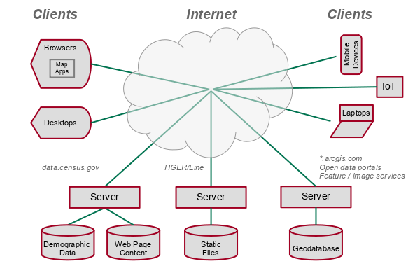
Feature Services
Feature services provide clients with access to vector features in a server geodatabase through REST endpoints.
- A REST endpoint is a URL to a service on the server that includes subfolders and parameters needed to identify a specific feature service.
- The acronym REST comes from the representational state transfer communications protocol used by these endpoints.
- Feature services allow you to access the most recently updated data on the server.
- Feature services are unstable because they are subject to updates or deletion at any time at the discretion of the feature service provider.
Data from feature service endpoints can be downloaded into your project geodatabase so you can preserve a snapshot of the current data in case the feature service data is modified or deleted.
- Downloading features in this manner can be unreliable, especially if you are downloading hundreds or thousands of features.
- If a link to a downloadable file is available, that may be a better option.
ArcGIS Online Feature Services
Numerous authors publish subsets of USCB data as feature services in ArcGIS Online. You should always use caution when accessing data from non-authoritative ArcGIS Online sources as the data is often work from student projects that is often of uncertain vintage and integrity.
The Minn 2019-2023 ACS feature service in the University of Illinois ArcGIS Online organization features a wide variety of commonly-used demographic variables from the 2019-2023 ACS five-year estimates data profile (DP) tables at state, county, and census tract aggregation levels. The data has full metadata and is also available as downloadable GeoJSON for use in R or Python.
Use the Export Features tool to copy the data from the feature service into the project geodatabase.
- Input Features: Browse into ArcGIS Online and search for the Minn 2019-2023 ACS feature service. Layers are available at the state, county, and census tract level. For this example, we use counties.
- Output Feature Class: Provide a meaningful name for the new feature class in the project geodatabase (Counties).
- Symbolize to make sure you have the variable you need.
Counties Filtered by State
If you only need counties in a specific state, you can use the Export Features tool with a filter.
- Input Features: Browse into ArcGIS Online and search for the Minn 2019-2023 ACS feature service. Layers are available at the state, county, and census tract level. For this example, we use counties.
- Output Feature Class: Provide a meaningful name for the new feature class in the project geodatabase (Counties).
- Filter Expression: In this example we filter by the ST state abbreviation field for counties in Illinois (IL).
- Symbolize to make sure you have the variable you need.
County Tracts Filtered by GEOID
Tracts for specific counties can be filtered using a GEOIDFQ, which is described above..
- Google the county name and FIPS code to find the five-digit FIPS code for the desired county. For this example, the FIPS code for Cook County, IL is 17031.
- Construct a GEOIDFQ prefix for the desired tracts. The GEOID for tracts begins with 1400000US, followed by the five digit county FIPS code, followed by the tract ID. Given the FIPS code found above, tract GEOIDs in Cook County begin with 1400000US17031.
- Use the Export Features tool to copy the tracts data from the feature service.
- Input Features: Browse ArcGIS Online for the feature service (Minn 2019-2023 ACS) and select the tracts layer.
- Output Feature Class: Browse to the project geodatabase and provide a name (Tracts).
- Filter Expression: Add a filter for GEOIDFQ begins with the GEOIDFQ prefix found above.
- Symbolize to make sure you have the variable you need.
Living Atlas Features
ESRI's Living Atlas of the World is a collection of geospatial data services that can be accessed in ArcGIS Pro or in ArcGIS Online. These services include data from the USCB and other government agencies.
Although the Living Atlas can be convenient, there are three issues with using Living Atlas data on a regular basis:
- Unclear: Ease of use obscures critical evaluation of the the original source and vintage of the data.
- Unstable: Living Atlas data is subject to change and deletion without notice.
- Unfree: Use of the Living Atlas encourages vendor lock-in.
You can download features from many Living Atlas feature services into your ArcGIS Pro project geodatabase.
- Open the Export Features tool.
- Input Features: Browse to the Living Atlas layer you want to download.
- Output Feature Class: Provide a meaningful name.
- Symbolize the new feature class by the desired variable.
Public Feature Services
Government agencies often make their geospatial data available through their open data portals.
- These portals occasionally provide links to feature services that are accessible to the general public, although they more commonly simply provide links to download the data as files.
- You can find these open data portals by Googling "name_of_place open data" or "name_of_place gis data."
In this example, we download the a feature class of trail center lines from the Lake County, IL Open Data & Records Hub.
- Acquire: Find the desired feature service and select I want to use this...
- Copy the GeoServer REST endpoint link from the API dropdown.
- Store: Under Analysis, Tools, open the
Export Features tool.
- Input Features: Copy the endpoint URL and remove the query component of the endpoint URL.
- Output Features: Browse into the project geodatabase and provide a meaningful name (Trails).
- Communicate: Symbolize as needed.
Data downloaded from feature services may cause the cryptic Geometry cannot have Z values error when packaging a project, even if the feature class properties do not indicate the presence of Z values. The workaround is to export the feature class to a shapefile, then export the shapefile back over the feature class in the project geodatabase.
ArcGIS Online
Using Precompiled Data
The video below demonstrates how to add the Minn 2015-2019 ACS Counties feature service available from the University of Illinois ArcGIS Online organization.
- Search for the layer in ArcGIS Online.
- If needed, resymbolize the layer and select the variable you wish to display. For this example we use median monthly rent.
- If needed, change the color ramp and/or adjust the scale to accentuate the differences.
- Change the blending mode to Multiply so you can see the base map as geographic context for your data.
- Save the map under a meaningful name (Minn County Income).
- Share the map.
- Copy the URL to get a link.
Living Atlas
The video below shows how to add a Living Atlas layer of median household income to a map in ArcGIS Online. Note that this layer is scale-dependent and changes the types of areas being displayed (states, counties, census tracts) depending on how closely you are zoomed in to the map.
- Create a new map in ArcGIS Online.
- Select Add and Living Atlas Layers.
- Search for the data by name, in this case median household income.
- Zoom in on the area you want to display. This particular layer is a scale-dependent layer that changes the types of areas displayed depending in how closely you are zoomed in to an area.
- Change the Blending to Multiply so you can see the base map and labels as geographic context for your data.
- Save the map under a meaningful name, share it, and copy the URL for a link (Minn_2019_County_Economics).
You can get metadata on the source and year of the information in a layer by opening the Properties panel and clicking on the link below Information.
Mapping Table Data in ArcGIS Online
For the join key, we use the USCB GEO_ID field that is common to both the table downloaded from data.census.gov and the TIGER/LINE shapefile.
- Download table data from data.census.gov as demonstrated above.
- Download an area polygon shapefile as demonstrated above.
- On your ArcGIS Online Content page, click New Item and upload the zipped shapefile as a hosted feature layer.
- Click New Item and upload the CSV as a hosted feature table.
- After the layer completes publishing, Open in Map Viewer.
- Click the Analysis icon on the right side panel and select Tools, Summarize Data, Join Features
- For the Target layer, select the layer created with the shapefile.
- For the Join layer, Browse layers and find the new table service.
- Under Attribute relationships, the target field will be AFFGEOID and the Join field will be GEO_ID.
- Under Result layer, give a meaningful Output name (Minn_2019_County_Economics).
- Estimate credits to make sure the operation will not use too many credits. County joins should use under 10 credits.
- Run. The join may take awhile depending on how many features you are joining. If the join takes longer than five minutes, the tool may have completed without notifying you. You can return to the home page, return to the map, and then add the layer from your content.
- Update the polygon Symbology based on the newly joined data variable
- Save the map under a meaningful title (Minn_2019_County_Economics).
- Back in your Content page, remove the original shapefile and table.
Table Data and TIGER Shapefiles
Zipped shapefiles can be read directly into the ArcGIS Online Map Viewer to create new feature classes for mapping and analysis.
Python
GeoPandas is a Python package for working with geospatial data.
Matplotlib is a Python package for plotting graphs.
Precompiled Data
To load precompiled ACS data into a GeoDataFrame in Python:
- Read the geospatial data from the file into a GeoDataFrame object using the read_file() function.
- The to_crs() method is used to reproject the data to the North America Lambert Conformal Conic projection suitable for North America (ESRI 102009).
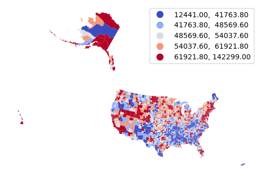
- The GeoDataFrame plot() method can be used to with the name of the attribute to visualize the variable as a choropleth map.
- The pyplot set_axis_off() method turns off the axis scale around the map, which is unnecessary with a projected map.
The pyplot show() function displays the plotted map.
import geopandas

import matplotlib.pyplot as plt

counties = geopandas.read_file("https://michaelminn.net/tutorials/data/2015-2019-acs-counties.geojson")

counties = counties.to_crs("ESRI:102009")

axis = counties.plot("Median Household Income", cmap = "coolwarm", legend=True, scheme="quantiles")

axis.set_axis_off()

plt.show()
We can filter the counties to show only the continental US to more effectively use the mapped area. We can also overlay a map of state outlines over the counties for geographic context.
counties = counties[~counties["ST"].isin(['AK', 'HI', 'PR'])]

states = geopandas.read_file("https://michaelminn.net/tutorials/data/2015-2019-acs-states.geojson")

states = states[~states["ST"].isin(['AK', 'HI', 'PR'])]

states = states.to_crs(counties.crs)

axis = counties.plot("Median Household Income", scheme="naturalbreaks",
	cmap="coolwarm_r", edgecolor="none", legend=True,
	legend_kwds={"bbox_to_anchor":(0.2, 0.4)})

states.plot(facecolor="none", edgecolor="#808080", ax=axis)

axis.set_axis_off()

plt.show()
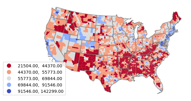
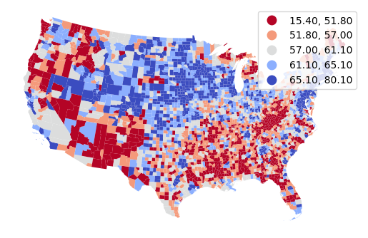
Table Data in Python
A conventional technique for acquiring USCB data is to download table data from data.census.gov and join it to TIGER polygons. Downloading is preferred over API access if you wish to preserve a snapshot of the data at a particular time, or you want to avoid the unreliability and download times associated with APIs.
- Download and clean up the table data as described above.
- Pandas is a Python package working with tabular data.
- GeoPandas is a Python package for working with geospatial data.
- Matplotlib is a Python package for plotting graphs.
- CSV files can be read into Pandas DataFrames using the read_csv() function.
- Find the URL to the appropriate TIGER cartographic boundary zipped shapefile from the link on the page shown above.
- Read the cartographic boundary file directly from the USCB website into a GeoDataFrame object using the read_file() function.
- Use the to_crs() method to reproject the data to the North America Lambert Conformal Conic projection suitable for North America (ESRI 102009).
- Join the table DataFrame with the county polygon GeoDataFrame using the Pandas merge() method and the GEO_ID fields in the two objects.
- To map only the continental 48 states, we exclude Alaska, Hawaii, and Puerto Rico using their FIPS codes.
import pandas

import geopandas

import matplotlib.pyplot as plt

county_data = pandas.read_csv("https://michaelminn.net/tutorials/gis-census/2023_County_Economics.csv")

counties = geopandas.read_file("https://www2.census.gov/geo/tiger/GENZ2019/shp/cb_2019_us_county_5m.zip")

counties = counties.to_crs("ESRI:102009")

counties = counties.merge(county_data, left_on="AFFGEOID", right_on="GEO_ID")

counties = counties[~counties["STATEFP"].isin(['02', '15', '72'])]

axis = counties.plot("Percent Workforce Participation", cmap="coolwarm_r", legend=True, scheme="quantiles")

axis.set_axis_off()

plt.show()
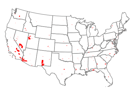
TIGER Shapefiles
- Find the URL to the appropriate TIGER cartographic boundary zipped shapefile from the link on the page shown above.
- Read the cartographic boundary file directly from the USCB website into a GeoDataFrame object using the read_file() function.
- The to_crs() method is used to reproject the data to the North America Lambert Conformal Conic projection suitable for North America (ESRI 102009).
- The GeoDataFrame plot() method plots the polygons.
- The pyplot set_axis_off() method turns off the axis scale that is unnecessary with a projected map.
- The pyplot show() function displays the plotted map.
import geopandas

import matplotlib.pyplot as plt

military = geopandas.read_file("https://www2.census.gov/geo/tiger/TIGER2023/MIL/tl_2023_us_mil.zip")

states = geopandas.read_file("https://www2.census.gov/geo/tiger/GENZ2023/shp/cb_2023_us_state_5m.zip")

states = states.to_crs("ESRI:102009")

military = military.to_crs("ESRI:102009")

axis = states.plot(facecolor='none', edgecolor='gray')

military.plot(facecolor='red', ax=axis)

axis.set_axis_off()

plt.show()
R
Functions from the sf (simple features) library are used to work with vector geospatial data in R.
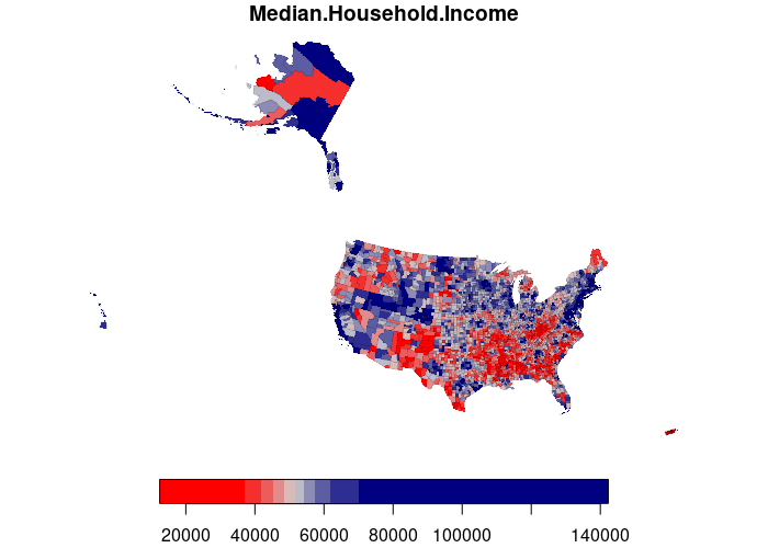
Precompiled Data
- Load the GeoJSON polygons into a simple features data.frame using st_read().
- Reproject the polygons into a cartographically appropriate projection with st_transform(). For this data we use the North America Lambert Conformal Conic projection suitable for North America (ESRI 102009).
- Create an appropriate diverging colorRampPalette.
- plot() a choropleth colored by the desired variable.
library(sf)

counties = st_read("https://michaelminn.net/tutorials/data/2015-2019-acs-counties.geojson")

counties = st_transform(counties, "ESRI:102009")

redblue = colorRampPalette(c("red", "lightgray", "navy"))

plot(counties["Median.Household.Income"], breaks="quantile", pal=redblue, lwd=0.1)
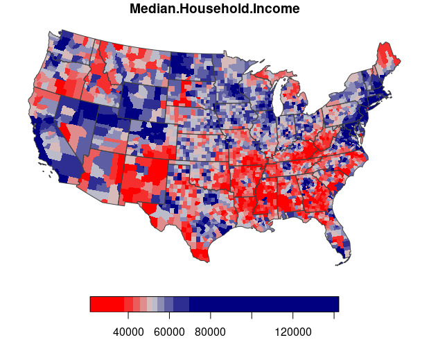
Filtering in R
We can filter the counties to show only the continental US to more effectively use the mapped area. We can also overlay a map of state outlines over the counties for geographic context.
states = st_read("https://michaelminn.net/tutorials/data/2015-2019-acs-states.geojson")

states = states[!(states$ST %in% c('AK', 'HI', 'PR')),]

states = st_transform(states, st_crs(counties))

counties = counties[!(counties$ST %in% c('AK', 'HI', 'PR')),]

plot(counties["Median.Household.Income"], breaks="quantile", pal=redblue, border=NA, reset=F)

plot(states$geometry, col=NA, border="#404040", add=T)
Shapefiles in R
- Load the shapefile polygons into a simple features data.frame using st_read().
- Although st_read() can read from URLs, it cannot process zipped shapefiles, so we need to use download.file() to download the files first.
- Adding /vsizip/ to the start of a file name will filter the zipped shapefiles through a virtual file system that exposes the shapefile contents to st_read().
- Reproject the polygons into a cartographically appropriate projection with st_transform(). For this data we use the North America Lambert Conformal Conic projection suitable for North America (ESRI 102009).
- To map only the continental 48 states, we exclude Alaska, Hawaii, and territories using their FIPS codes.
library(sf)

download.file('https://www2.census.gov/geo/tiger/TIGER2023/MIL/tl_2023_us_mil.zip', 'temp.zip')

military = st_read('/vsizip/temp.zip')

download.file('https://www2.census.gov/geo/tiger/GENZ2023/shp/cb_2023_us_state_5m.zip', 'temp.zip')

states = st_read('/vsizip/temp.zip')

military = st_transform(military, "ESRI:102009")

states = st_transform(states, "ESRI:102009")

states = states[!(states$STATEFP %in% c('02', '15', '60', '66','69', '72', '78')),]

plot(states$geometry, col=NA, border='gray')

plot(military$geometry, col='red', add=T)
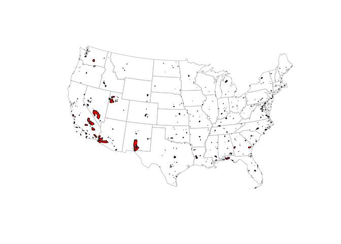
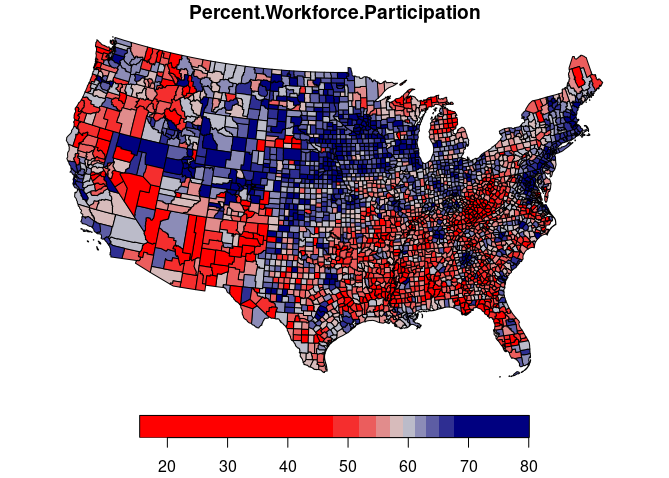
Table Data in R
A conventional technique for acquiring USCB data is to download table data from data.census.gov and join it to TIGER polygons. Downloading is preferred over API access if you wish to preserve a snapshot of the data at a particular time, or you want to avoid the unreliability and download times associated with APIs.
- Download and clean up the table data as described above.
- Read the table data into an R data.frame using the read.csv() function.
- Find the URL to the appropriate TIGER cartographic boundary zipped shapefile from the link on the page shown above.
- download.file() to a temporary file with the .shz extension. You must go through this intermediate step so the file has the .shz extension so that st_read() knows this is a zipped shapefile.
- Load the shapefile polygons into a simple features data.frame using st_read().
- Reproject the polygons into a cartographically appropriate projection with st_transform(). For this data we use the North America Lambert Conformal Conic projection suitable for North America (ESRI 102009).
- merge() the polygons and the table on the GEO_ID fields.
- To map only the continental 48 states, we exclude Alaska, Hawaii, and Puerto Rico using their FIPS codes.
- Create an appropriate diverging colorRampPalette.
- plot() a choropleth colored by the desired variable.
library(sf)

county_data = read.csv("https://michaelminn.net/tutorials/gis-census/2023_County_Economics.csv")

download.file("https://www2.census.gov/geo/tiger/GENZ2019/shp/cb_2019_us_county_5m.zip", "temp.shz")

counties = st_read("temp.shz")

counties = st_transform(counties, "ESRI:102009")

counties = merge(counties, county_data, by.x="AFFGEOID", by.y="GEO_ID")

counties = counties[!(counties$STATEFP %in% c('02', '15', '72')),]

redblue = colorRampPalette(c("red", "lightgray", "navy"))

plot(counties["Percent.Workforce.Participation"], pal=redblue, breaks="quantile")
If you want to save a copy of your processed data for later use, you can use the st_write() function to create a variety of different types of geospatial data files.
st_write(counties, "2019_County_Economics.geojson")
The US Census Bureau API
The USCB makes much of their data available through application programmers interfaces (APIs) that permit direct access to current versions of USCB data via services.
Although APIs have a learning curve, if you are using USCB data in R or Python, access through an API can be a much more flexible way of accessing USCB data than manually downloading and cleaning table data.
ACS Variables
ACS variables are referenced by cryptic variable names that indicate the source table and the number of the variable in that table, along with letters that indicate whether the variable represents estimated values or margins of error. Adding to the complexity, variables representing different types of summarization are stored in different reference files.
For this example, we focus on data from the 2015-2019 ACS five-year estimates that represent the final data release reflecting the pre-COVID world.
Typical variables from the profile variable list (DP02 - DP05) include:
- DP02_0016E: Average household size
- DP02_0065PE: Percent bachelor's degree
- DP02_0066PE: Percent graduate degree
- DP02_0070PE: Percent veterans
- DP02_0093PE: Percent foreign born
- DP03_0025E: Mean minutes to work
- DP03_0062E: Median household income
- DP04_0003PE: Percent vacant units
- DP04_0046PE: Percent homeowners
- DP04_0047PE: Percent renters
- DP04_0089E: Median home value
- DP04_0101E: Median monthly mortgage costs
- DP04_0134E: Median rent
- DP05_0018E: Median age
Typical variables from the subject variable list include:
- S0101_C01_001E: Total population
- S0101_C01_002E: Population under 5
- S0101_C01_022E: Population under 18 years
- S0101_C01_030E: Population 65 years or over
- S0801_C01_003E: Percent drive alone to work
- S0801_C01_009E: Percent transit to work
- S0801_C01_013E: Percent work at home
- S1301_C05_001E: Percent single mothers
- S1301_C04_001E: Annual births per 1K women
- S2504_C02_027E: Percent of homes with no vehicle
API Calls
USCB API calls are URLs with path components and parameters that will return the requested data. This list of available APIs describes the different API options.
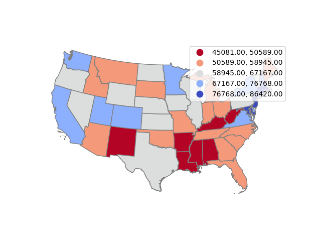
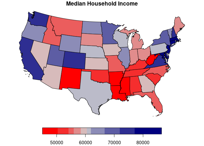
For this examples, we will download state-level median household income (DP03_0062E) from the 2015-2019 ACS five-year estimates that represent the final data release reflecting the pre-COVID world.
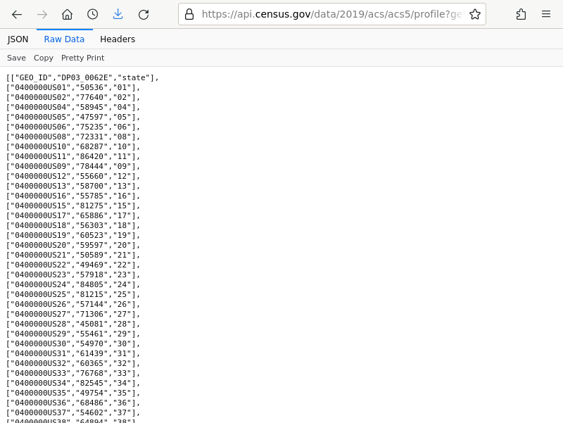
For this API query URL:
https://api.census.gov/data/2019/acs/acs5/profile?get=GEO_ID,DP03_0062E&for=state:*
- The path for profile variables is https://api.census.gov/data/2019/acs/acs5/profile
- The get= parameter is a list of requested variable names.
- The GEO_ID variable is the GEOID needed for the join with the TIGER polygons (below).
- The for= parameter indicates the FIPS code(s) for the desired areas. Wildcards (*) can be specified
- An optional key= parameter specifies the API key (if needed for high volume applications).
Using USCB API Data in Python
To create a GeoDataFrame of ACS data:
- GeoPandas is a Python package for working with geospatial data.
- Matplotlib is a Python package for plotting graphs.
- Load the API data into a DataFrame by passing the API URL to the Pandas read_json() function.
- Use iloc to remove the header row and the redundant state column.
- rename() the columns with meaningful names.
- astype(float) to convert the data column from text to numeric.
- Find the URL to the appropriate TIGER cartographic boundary zipped shapefile from the link on the page shown above.
- Read the cartographic boundary file directly from the USCB website into a GeoDataFrame object using the read_file() function.
- Use the to_crs() method to reproject the data to the North America Lambert Conformal Conic projection suitable for North America (ESRI 102009).
- Join the table DataFrame with the county polygon GeoDataFrame using the Pandas merge() method and the GEO_ID fields in the two objects.
- To map only the continental 48 states, we exclude Alaska, Hawaii, and Puerto Rico.
import pandas

import geopandas

import matplotlib.pyplot as plt

state_income = pandas.read_json("https://api.census.gov/data/2019/acs/acs5/profile?get=GEO_ID,DP03_0062E&for=state:*")

state_income = state_income.iloc[1:, 0:2]

state_income = state_income.rename(columns={0:"GEO_ID", 1:"Median Household Income"})

state_income.iloc[:,1] = state_income.iloc[:,1].astype(float)

states = geopandas.read_file("https://www2.census.gov/geo/tiger/GENZ2022/shp/cb_2022_us_state_5m.zip")

states = states.to_crs("ESRI:102009")

state_income = states.merge(state_income, left_on="AFFGEOID", right_on="GEO_ID")

state_income = state_income[~state_income["STUSPS"].isin(['AK', 'HI', 'PR'])]

axis = state_income.plot("Median Household Income", scheme="naturalbreaks",
	cmap="coolwarm_r", edgecolor="#808080", legend=True)

axis.set_axis_off()

plt.show()
County Level Data
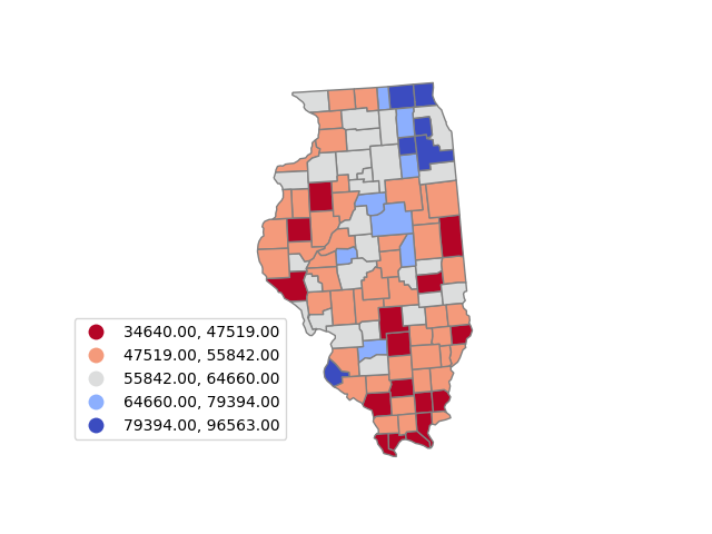
County level data can be loaded by modifying the API parameters and joining with the TIGER counties file.
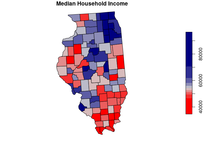
This example maps median household income (DP03_0062E) by Illinois county (state FIPS 17).
county_income = pandas.read_json("https://api.census.gov/data/2019/acs/acs5/profile?get=GEO_ID,DP03_0062E&for=county:*&in=state:17")

county_income = county_income.iloc[1:, 0:2]

county_income = county_income.rename(columns={0:"GEO_ID", 1:"Median Household Income"})

county_income.iloc[:,1] = county_income.iloc[:,1].astype(float)

counties = geopandas.read_file("https://www2.census.gov/geo/tiger/GENZ2019/shp/cb_2019_us_county_20m.zip")

counties = counties.to_crs("ESRI:102009")

county_income = counties.merge(county_income, left_on="AFFGEOID", right_on="GEO_ID")

axis = county_income.plot("Median Household Income", scheme="naturalbreaks",
	cmap="coolwarm_r", edgecolor="#808080", legend=True,
	legend_kwds={"bbox_to_anchor":(0.2, 0.4)})

axis.set_axis_off()

plt.show()
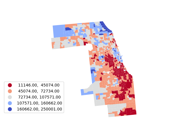
Tract-Level Data
Census tracts are subdivisions of counties that are drawn based on clearly identifiable features to ideally contain around 4,000 residents, although in practice the range of population is usually between 1,200 and 8,000 (USCB 2019).
This example maps median household income (DP03_0062E) by census tract in Cook County, Illinois (state FIPS 17, county FIPS 031).
Note that tract-level data is commonly undisclosed or unavailable and is represented with the negative number -666666666. This code resets those values to zero to avoid distorting the legend.
tract_income = pandas.read_json("https://api.census.gov/data/2019/acs/acs5/profile?get=GEO_ID,DP03_0062E&for=tract:*&in=state:17&in=county:031")

tract_income = tract_income.iloc[1:, 0:2]

tract_income = tract_income.rename(columns={0:"GEO_ID", 1:"Median Household Income"})

tract_income.iloc[:,1] = tract_income.iloc[:,1].astype(float)

tract_income[tract_income["Median Household Income"] < 0] = 0

tracts = geopandas.read_file("https://www2.census.gov/geo/tiger/GENZ2019/shp/cb_2019_17_tract_500k.zip")

tracts = tracts.to_crs("ESRI:102009")

tract_income = tracts.merge(tract_income, left_on="AFFGEOID", right_on="GEO_ID")

axis = tract_income.plot("Median Household Income", scheme="naturalbreaks",
	cmap="coolwarm_r", edgecolor="none", legend=True,
	legend_kwds={"bbox_to_anchor":(0.2, 0.4)})

axis.set_axis_off()

plt.show()
Using USCB API Data in R
To create a data.frame of ACS data:
- The sf (simple features) library provides functions for working with vector geospatial data.
- The jsonlite library is a JSON parser.
- Load API data as a data.frame by passing the API URL to the jsonlite fromJSON() function.
- Remove the header row and the redundant state column.
- Provide meaningful column names().
- Use as.numeric() to convert the data column from text to numeric.
- Find the URL to the appropriate TIGER cartographic boundary zipped shapefile from the link on the page shown above.
- download.file() to a temporary file with the .shz extension. You must go through this intermediate step so the file has the .shz extension so that st_read() knows this is a zipped shapefile.
- Load the shapefile polygons into a simple features data.frame using st_read().
- Reproject the polygons into a cartographically appropriate projection with st_transform(). For this data we use the North America Lambert Conformal Conic projection suitable for North America (ESRI 102009).
- merge() the polygons and the table on the GEO_ID fields.
- To map only the continental 48 states, we exclude Alaska, Hawaii, and Puerto Rico using their FIPS codes.
- Create an appropriate diverging colorRampPalette.
- plot() a choropleth colored by the desired variable.
library(sf)

library(jsonlite)

state_data = fromJSON("https://api.census.gov/data/2019/acs/acs5/profile?get=GEO_ID,DP03_0062E&for=state:*")

state_data = as.data.frame(state_data[2:nrow(state_data),1:2],)

state_data[,2] = as.numeric(state_data[,2])

names(state_data) = c("GEO_ID", "Median Household Income")

download.file("https://www2.census.gov/geo/tiger/GENZ2022/shp/cb_2022_us_state_5m.zip", "temp.shz")

states = st_read("temp.shz")

states = st_transform(states, "ESRI:102009")

state_income = merge(states, state_data, by.x="AFFGEOID", by.y="GEO_ID")

state_income = state_income[!(state_income$STUSPS %in% c('AK', 'HI', 'PR')),]

redblue = colorRampPalette(c("red", "lightgray", "navy"))

plot(state_income["Median Household Income"], pal=redblue, breaks="quantile")
County Level Data
County level data can be loaded by modifying the API parameters and joining with the TIGER counties file.
This example maps median household income (DP03_0062E) by Illinois county (state FIPS 17).
county_data = fromJSON("https://api.census.gov/data/2019/acs/acs5/profile?get=GEO_ID,DP03_0062E&for=county:*&in=state:17")

county_data = as.data.frame(county_data[2:nrow(county_data),1:2],)

county_data[,2] = as.numeric(county_data[,2])

names(county_data) = c("GEO_ID", "Median Household Income")

download.file("https://www2.census.gov/geo/tiger/GENZ2019/shp/cb_2019_us_county_20m.zip", "temp.shz")

counties = st_read("temp.shz")

counties = st_transform(counties, "ESRI:102009")

county_income = merge(counties, county_data, by.x="AFFGEOID", by.y="GEO_ID")

redblue = colorRampPalette(c("red", "lightgray", "navy"))

plot(county_income["Median Household Income"], pal=redblue, breaks="quantile")
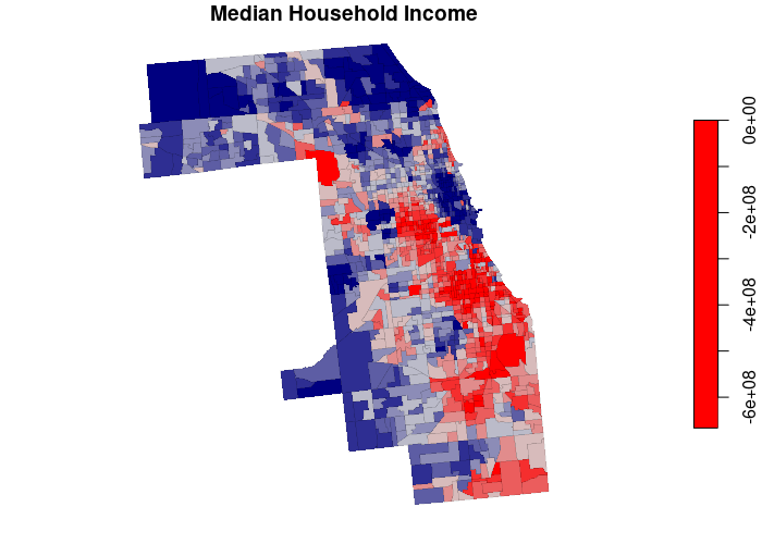
Tract-Level Data
Census tracts are subdivisions of counties that are drawn based on clearly identifiable features to ideally contain around 4,000 residents, although in practice the range of population is usually between 1,200 and 8,000 (USCB 2019).
This example maps median household income (DP03_0062E) by census tract in Cook County, Illinois (state FIPS 17, county FIPS 031).
Note that tract-level data is commonly undisclosed or unavailable and is represented with the negative number -666666666. This code resets those values to zero to avoid distorting the legend.
tract_data = fromJSON("https://api.census.gov/data/2019/acs/acs5/profile?get=GEO_ID,DP03_0062E&for=tract:*&in=state:17&in=county:031")

tract_data = as.data.frame(tract_data[2:nrow(tract_data),1:2],)

tract_data[,2] = as.numeric(tract_data[,2])

names(tract_data) = c("GEO_ID", "Median Household Income")

download.file("https://www2.census.gov/geo/tiger/GENZ2019/shp/cb_2019_us_tract_500k.zip", "temp.shz")

tracts = st_read("temp.shz")

tracts = st_transform(tracts, "ESRI:102009")

tract_income = merge(tracts, tract_data, by.x="AFFGEOID", by.y="GEO_ID")

redblue = colorRampPalette(c("red", "lightgray", "navy"))

plot(tract_income["Median Household Income"], pal=redblue, breaks="quantile", lwd=0.1)