Areas
Rev. 2 February 2025
A classic means of organizing space, both in the material world and in geographic information systems, is division of land into areas.
There are a variety of different types of areas used for different types of management and analysis. Those areas can be identified with a variety of different naming and numbering schemes. Areas are commonly visualized as maps and analysis of the distribution patterns of attributes across areas is one of the classical techniques of geography. Those will be the subjects of this tutorial.
Polygons
An area is "a particular extent of space or surface" (Merriam-Webster 2020).
Areas are usually represented in GIS with vector polygons.
Polygons are formed by connecting node points at specific latitudes and longitudes with edge lines that form boundaries.
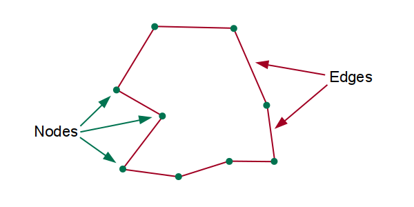
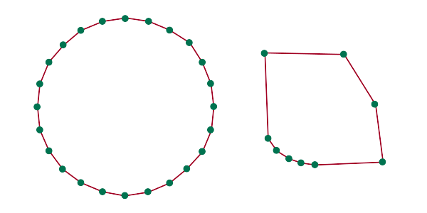
Curved boundaries are usually stored in GIS as polygons using closely spaced nodes that appear as curves when viewed. Conventional GIS data models do not have the ability to represent complex geometric representations (such as Bézier curves) that are available in graphic design programs like Illustrator.
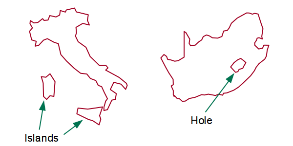
Individual features sometimes consist of multiple polygons that are treated a single entity in GIS. In the example below, the border of England includes islands off the coast. In the second example, the country of South Africa wraps around the country of Lesotho, and the border of Lesotho is a second polygon carving out a hole in the contiguous area of the country.
Human-defined areas such as political boundaries or building footprints are discrete phenomena with clearly defined edges that are usually best represented as vector polygon objects.
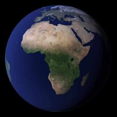
However, some phenomena, especially environmental phenomena, are continuous phenomena that often do not have clear boundaries and are best represented as rasters. In the example raster below, there are clearly areas of high and low vegetation across Africa, but those levels vary continuously across the landscape.
Types of Areas
Getis et al. (2014, 14) defined a taxonomy of four different types of regions that expanded on Hartshorne's (1959) original three-part taxonomy. In the world of GIS, this taxonomy is useful for understanding these different types of areas and how information about them can best be captured, analyzed, and communicated.
- Administrative areas
- Formal areas
- Functional areas
- Vernacular areas
Administrative Areas
Administrative areas are areas that are "created by laws, treaties, or regulations" and are usually associated with government, military, or business control or operation (Getis et al. 2014, 14).
Administrative areas have clear, rigorously surveyed boundaries that are well-represented by discrete object polygons.
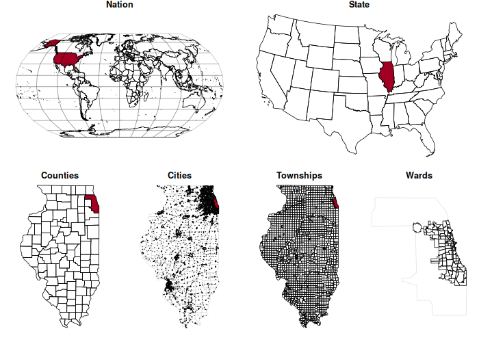
In the United States, there is a rough nested hierarchy of administrative areas that divide the country into areas that are managed by different levels of government:
- The nation is an area enclosed in country boundaries defined by international agreement.
- States are the 50 governmental areas in the US federal system with historically defined legal boundaries.
- Counties are the largest territorial division of states for local government in the US.
- Townships are area subdivisions of counties, and the organization of these varies by state. Townships are often associated with unincorporated areas of counties.
- Cities are municipal corporations incorporated and governed under a charter granted by the state.
- Wards and city council districts are subdivisions of cities often represented by officials elected from those wards / districts.
Local Administrative Areas
At the local level, there is a much wider range of different areas used to divide cities into manageable chunks overseen by separate administrators and departments, such as:
- Boroughs
- Police Precincts
- Voting Precincts
- Health Districts
- School Districts
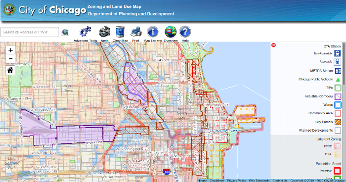
Land use zones are an especially complicated type of administrative area that govern the types of buildings and businesses that can operate in particular areas of cities. The boundaries are dictated by a variety of political and economic factors.
Cadastres
A cadastre is "an official register of the quantity, value, and ownership of real estate used in apportioning taxes" (Merriam-Webster 2020).
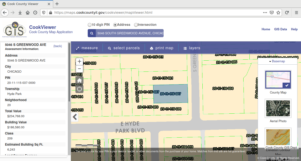
- Parcels are clearly defined areas of property ownership.
- Counties commonly use GIS that represent parcels in a cadastre as polygons.
- City GIS technicians and analysts maintain cadastres based on the work of surveyors and assessors.
Data commonly included in a cadastre includes:
- Property id number
- Street address, city, state, zip
- Owner name and address
- Acreage
- Assessed land, building, farmland, and farm building value
- Deed information
- PLSS section, township, range
Assessed values are used for calculating property taxes and often vary significantly from market value (Bond 2022). Homes of low-income residents are often assessed more aggressively, resulting in higher tax rates for those residents relative to residents of wealthier neighborhoods (Srikanth 2021).
Census Tracts
The US Census Bureau (USCB) is the part of the US federal government responsible for collecting data about people (demographics) and the economy in the United States. The Census Bureau has its roots in Article I, section 2 of the US Constitution, which mandates an enumeration of the entire US population every ten years (the decennial census) in order to set the number of members from each state in the House of Representatives (the lower house of the US Congress) and Electoral College (that selects the US President) (USCB 2017).
To preserve the privacy of people who respond to the census or other surveys run by the USCB, the USCB only releases data to the public that has been aggregated to areas. The smallest areas of data that the USCB releases data in are census tracts and, sometimes, block groups. Accordingly, data by census tract provides a fine-grained GIS view of community demographics that is very useful in social and economic research.
Census tracts are subdivisions of counties that are drawn based on clearly identifiable features to ideally contain around 4,000 residents, although in practice the range of population is usually between 1,200 and 8,000 (USCB 2019).
Formal Areas
Formal areas (uniform regions) are areas that each have a common set of physical or social characteristics.
Although Hartshorne's (1959) original taxonomy considered administrative areas to simply be a specific type of formal areas, this tutorial follows Getis et al. (2014, 14) in seeing formal areas as defined by their contents rather than by the decisions of governing authorities.
One challenge of this approach is that in the absence of a clear authority to specify the exact boundaries of formal areas, the boundaries can be ambiguous and/or contested.
For example, social scientists often make a distinction between nations and states. Nations are groups of people that have a common identity, often based on common history, religion, or social practices. In contrast, a state (country) is a governmental entity that controls a specific geographical area. This definition should not be confused with the use of the term state in the US to represent one of the 50 United States that are part of the federal system of government.
While governments usually strive to create a national identity within their borders, different geographic parts of states can be home to different nations. Conflicts between different nations within states often result in violent civil war and / or violent efforts by the state to suppress national identities that conflict with the state.
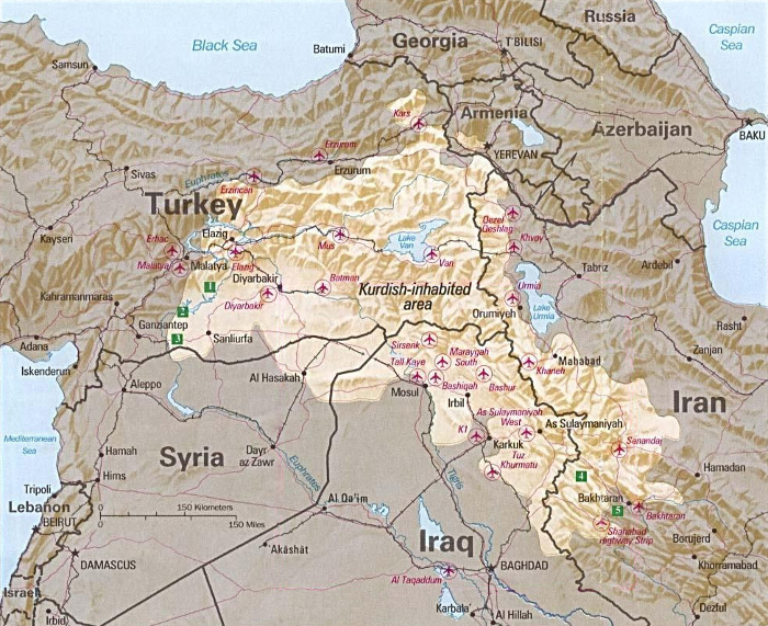
Such an example is Kurdistan. The Kurds are an ethnic group distributed across a largely contiguous area that falls within the states of Turkey, Syria, Iraq, and Iran. Many Kurds (Kurdish nationalists) aspire to to create an independent Kurdish state, which has resulted in often violent suppression by existing state governments that do not want to lose control of the territory that would form that independent state.
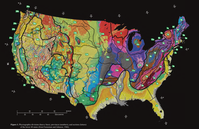
Similarly, areas of different environmental characteristics can be considered formal areas. For example, physiographic regions are areas classified by common geological structures and histories based on a taxonomy initially developed by Nevin Fenneman (1917).
Functional Areas
Functional areas (nodal regions) are focused on a central point, with diminishing influence the further you go away from that central point.
Metropolitan areas are functional areas that include "a major city together with its suburbs and nearby cities, towns, and environs over which the major city exercises a commanding economic and social influence" (Encyclopedia Britannica 2020). Metropolitan functional area boundaries often cross multiple city, county, and state administrative boundaries.
For tabulating purposes, the US Census Bureau defines a set of administrative areas as core-based statistical areas (CBSA) that include metropolitan statistical areas (big cities) and micropolitan statistical areas (small cities).
Although the USCB distributes information about metropolitan areas as clear boundaries in shapefiles, different types of influence (such as access to health care or commuting distances) can have different extents, and ties to the global economy can spread influence worldwide. Accordingly, you should interpret maps of functional areas with this ambiguity in mind.
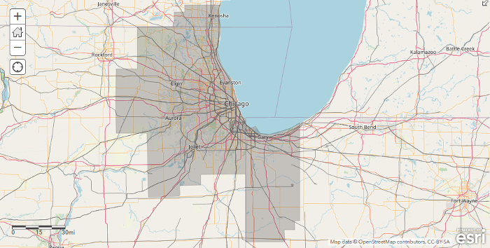
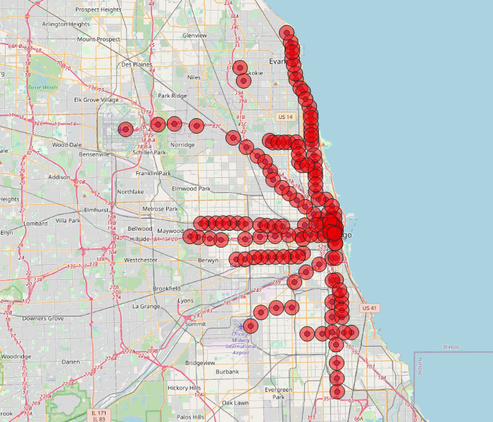
Another common example of functional areas used in urban transportation planning are areas within walking distance of transit stops. In the map below, the red circles encompass areas within a 1/2 mile of stations on the CTA El rail lines.
Vernacular Areas
Vernacular areas (perceptual regions) are areas that are socially-defined by shared history and common identities (Wikipedia 2020).
An example of a vernacular area is a neighborhood, which is "a residential section of a city" (Merriam-Webster 2020).
Neighborhood boundaries are inexact because they are defined by identities that are subjective and evolve over time under the influence of ethnic groups, real estate developers, and urban planners (city government). Neighborhoods grow and shrink based on time and social attitudes. Residents in adjacent homes may think of themselves as living in different neighborhoods even if there are no clear physical markers to indicate any difference between the neighborhood identity of their properties.
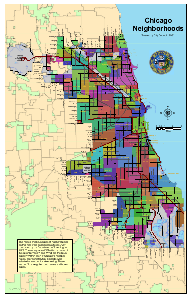
City governments often create maps showing clear neighborhood boundaries for planning purposes, but some residents of those neighborhoods may have a different opinion of which neighborhood they belong in. For example, this neighborhood map created by the City of Chicago was based on a field survey from 1978 asking randomly selected residents what neighborhood they lived in:
Area Identifiers
Names
Once a set of areas have been defined, you need a way of identifying individual areas. Perhaps the most common way of identifying specific areas is with names. Countries have names, cities have names, and neighborhoods have names.
A challenge of using names with geographic information systems is that GIS uses coordinate systems (usually latitude and longitude) to represent locations. Names often do not uniquely identify a specific latitudes and longitudes on the surface of the planet.
The process of converting place names to latitudes and longitudes is called geocoding. This requires large databases and complex algorithms to deal with the idiosyncrasies of place names, such as:
- Multiple areas with the same names
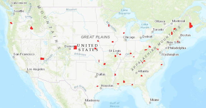
- There are 28 different Washington Counties in the US
- There are two different Salem, MO
- Abbreviations and punctuation differences
- St. George vs. St George vs. Saint George
- DC vs. D.C. vs. the District of Columbia
- Similar names
- Democratic Republic of the Congo vs. Republic of the Congo vs. the Congo River
- The Republic of Korea (South Korea) vs. the Democratic People's Republic of Korea (North Korea)
- Formal vs. common names
- Iran vs. the Islamic Republic of Iran
- China vs. the People's Republic of China
- Language differences
- Federal Republic of Germany vs. Bundesrepublik Deutschland
- People's Republic of China vs. 中华人民共和国
- Areas split and merge under similar names
- The German Reich was split into the Federal Republic of Germany (West Germany) and the German Democratic Republic (East Germany) after WW II, then reunified into the Federal Republic of Germany in 1991.
- Czechoslovakia separated from the Austro-Hungarian Empire in 1918, and then split into the Czech Republic and Slovakia in 1993.
- Name changes over time
- The Sears Tower (1973) vs. The Willis Tower (2009)
- Comiskey Park (1991) vs. US Cellular Field (2003) vs. Guaranteed Rate Field (2016)
Latitudes and Longitudes
The polygons used to represent discrete areas are created using points at specific latitudes and longitudes that are connected using lines. In some cases, one feature may contain multiple polygons for things like separate islands, or to represent holes in polygons, such as for bodies of water.
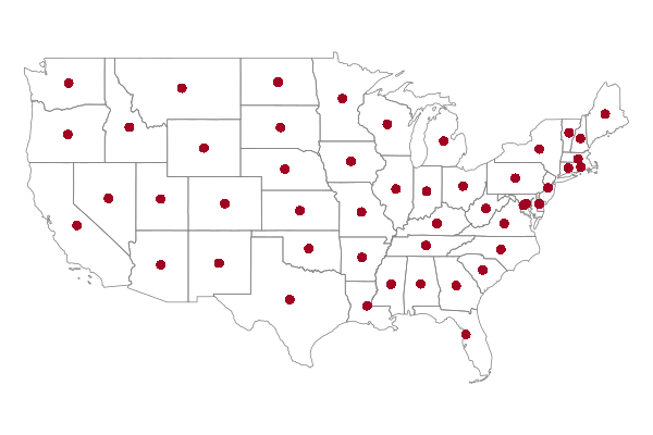
To simplify identification of areas, these collections of points are often generalized into a single point. This is a common practice with GPS apps when giving directions from one area to another.
These points can be placed at entrances to areas, such as doorways or front gates. However, a more common technique is to place points at centroids, which are locations within polygons that are the geometric center of mass of the polygon.
Linear Addresses
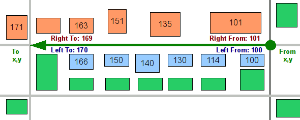
Linear addresses are location identifiers based on a named streets and additional identifier(s) that specify specific locations on those streets. Locations in urban areas are commonly identified with linear addresses, although the standard formats of these addresses vary widely by country, and addressing standards within countries can have a significant amount of variation.
In the United States:
- The common format for street addresses is a number followed by a street name: 101 Main Street.
- Individual apartments or offices at a single street address are often followed by a suite number: 101 Main Street #204.
- The street address then needs an additional city and state name to distinguish it from identical street addresses in other cities: 101 Main Street, Peoria, IL
- Linear addresses are commonly used by the US Post Office for specifying destinations for packages and letters sent by mail.
As with place names, street addresses have multiple challenges that make the geocoding of addresses into latitudes and longitudes difficult and imperfect:
- Street numbers can have additional punctuation or lettering.
- Streets can have multiple names: Sixth Avenue vs. Avenue of the Americas in New York City
- There an be multiple streets of with the same name in a city.
- Streets are often divided into east and west sections.
- Street names are sometimes changed over time.
- Street numbers are sometimes moved.
- Place names are sometimes used instead of street names: One Bryant Park
- Street names have a variety of different abbreviations and punctuations: First ST, 1st St., 1st Street
- Typographical errors are common with addresses.
- Different countries use radically different address schemes from the US.
Standardized Codes
The ambiguity associated with place names and linear addresses can be resolved by using standardized coding systems that uniquely identify areas and other types of locations.
ISO Country Codes
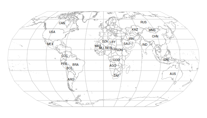
At the international level, the International Organization for Standardization (ISO) has defined two-letter and three-letter country codes (ISO 3166-1 alpha-2 and alpha-3) that uniquely identify past and current country boundaries. These codes mitigate some of the challenges associated with country names as place names that were described above.
Zip Codes
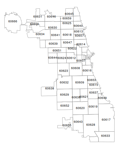
The US Postal Service divides the country into delivery service administrative areas that are identified with five-digit zip codes. Postal systems in most countries of the world also have similar areas, albeit with different ways of identifying those areas. These codes are used when physically mailing letters or packages.
The ZIP in zip code is an acronym for Zone Improvement Plan that was "introduced July 1, 1963, as part of a larger Postal Service Nationwide Improved Mail Service (NIMS) plan to improve the speed of mail delivery" (Library of Congress 2021). Acronyms commonly shift to lower case after a period of frequent use (CMS 2017, 10.6), and Merriam-Webster (2022) and the Chicago Manual of Style (2017, 10.29) favor fully-lowercase. However, the US Government Publishing Office Style Manual (2016) retains the fully-uppercase acronym capitalization.
FIPS Codes
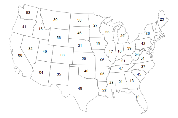
The United States Federal Information Processing Standards (FIPS) included a set of two-digit state codes (FIPS 5-1 from 1970 and FIPS 5-2 from 1987) and five-digit county codes (FIPS 6-4 from 1990). In 2008, the management of the standard moved from the National Institutes of Standards to ANSI's InterNational Committee for Information Technology Standards, with the county code standard becoming INCITS 31-2009 (US Census Bureau 2020).
The US Census Bureau's GEOID coding system is used to uniquely identify various geographic units in its data files based on these standards, and preserves the FIPS acronym (US Census Bureau 2020).
- States: two-digit codes
- Counties: five-digit code comprised of the two-digit state code followed by a three-digit county code
- Census Tract: 11-digit code comprised of the five-digit county code followed by a six-digit tract code
Local Codes
Local governments use a wide variety of idiosyncratic identifier codes for parcels and structures.
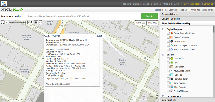
For example, the City of New York's Property Land Use Tax lot Output (PLUTO) system organizes parcels (individual areas of owned land) by block and lot numbers.
Uncertainty
Data is a simplified abstraction that represents the infinitely-complex real world. The process of capturing data by translating the real world into an abstraction always introduces some level of uncertainty about the correspondence of our data to the facts on the ground.
Uncertainty means that something is "not clearly identified or defined" (Merriam-Webster 2021). While the rigorous computational technology of GIS implies absolute truth, uncertainty means that you need to interpret geospatial data with an understanding that the data may deviate from the actual ground truth, or the representations of that data may give a mistaken impression of the actual ground truth.
Since the outputs of GIS are often used to guide decision-making, it is important for the GIS professional to communicate uncertainty so the decision-makers understand the limitations of the information they have been given. Failure to do this can be an ethical issue that can result in harm. Negligence in adhering to professional protocols can result in legal liability.
Longley et al. (2015, 99 - 127) define three levels of uncertainty in geospatial data that are particularly relevant when working with areas: conception, representation, and analysis.
Conceptual Uncertainty
The abstract polygons used to represent areas have exact nodal coordinates and clear lines. Administrative areas usually have stable, rigorously surveyed borders that both lend themselves to representation in GIS and demand use of GIS to preserve accuracy.
However, the borders of formal, functional, and vernacular areas are often less clear. In order to draw borders around a phenomenon you need to be able to classify it into specific categories that will form clear boundaries. Such clarity is often unavailable because categories all have some measure of the following qualities:
- Vague: Categories can be vague, where the exact definition of a category is unclear. An example is soil types that require arbitrary criteria to separate different classifications.
- Ambiguous: Membership in categories can ambiguous, where it is unclear which categories a part of an area belongs to. An example is the aforementioned neighborhoods where people are often uncertain about what neighborhood they do/should belong in.
- Contested: Even when criteria are clear, membership in categories is subject to debate and conflict, such as with the example of Kurdistan above being fought over by a variety of political actors.
- Dynamic: Geospatial data is usually a static snapshot in time, but most phenomena change over time. Parts of a data set can become outdated before the resources are available to revise them.
- Incomplete: Geospatial data is often sampled, where statistical inferences about the larger population are made based on capture of a limited set of data. Accuracy can be expressed as margins of error, but those values are often ignored (as with political polling) and 100% confidence is impossible with sampled data.
Representational Uncertainty
The way in which geospatial data is stored in GIS can add additional uncertainty.
- Accuracy vs. precision: Numeric values for coordinates and attributes are usually represented in computers using floating-point numbers that can store values with a high number of significant digits. However, our spatial or attribute measurements are usually estimates or rough measures where we can only be certain of accuracy to three or four significant digits. Therefore, there is often a conflict between what we know (accuracy) and how we say it (precision) For example, the default precision in legends in ArcGIS Pro is to six decimal places. However, our data is rarely that accurate, and the use of the extra decimal places on maps dramatically overstates the level of accuracy that is available.
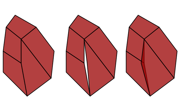
- Topological errors: Areas are represented in GIS as polygons. Polygons in a data set are often hand drawn and / or come from different sources. This frequently results in errors where the edges of adjacent polygons either overlap or fail to meet, resulting in slivers. GIS software has tools to adjust the nodes in polygons to fix these problems, although the fixes then introduce the question of whether the moved border(s) comport with reality.
Analytical Uncertainty
Different choices of what types and boundaries of areas you used to aggregate spatial data can result in radically different results.
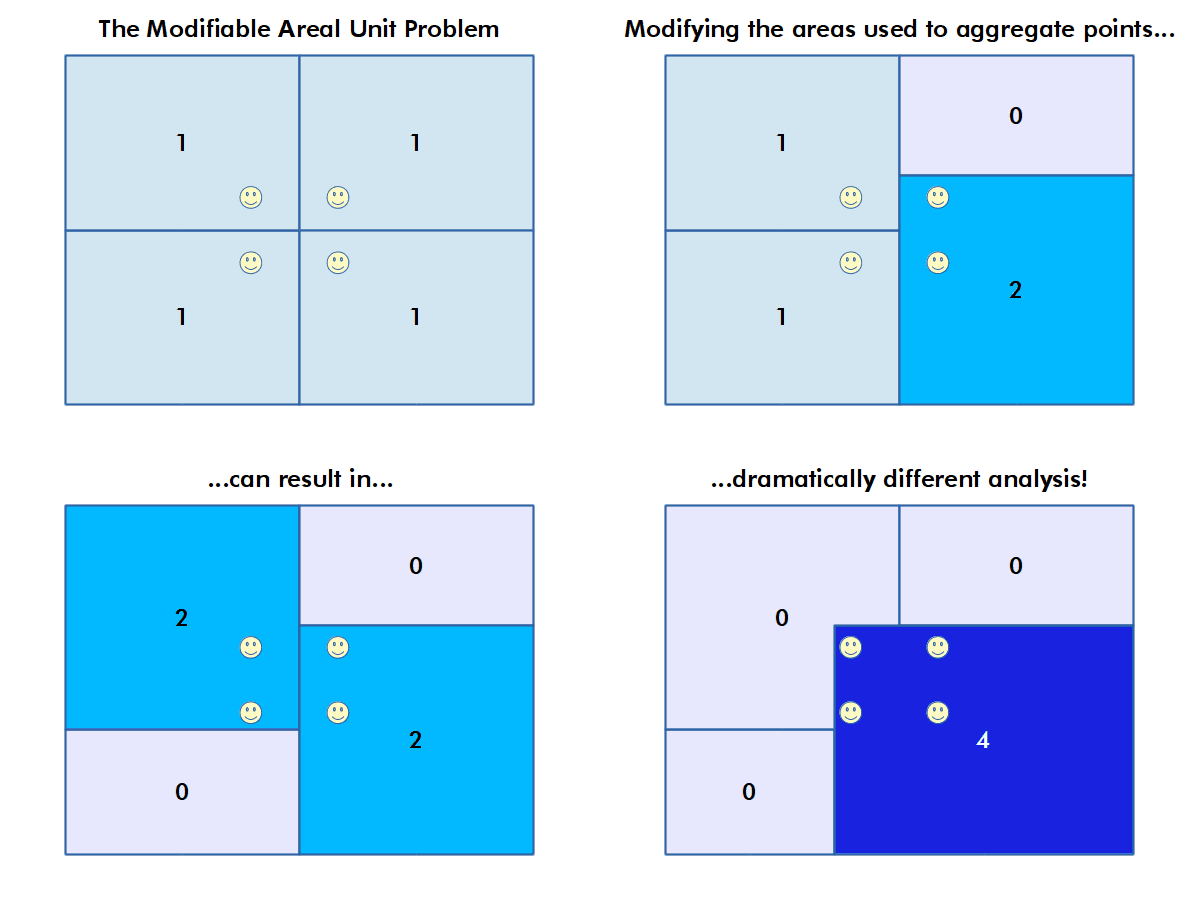
The modifiable areal unit problem (MAUP) is "a source of statistical bias that is common in spatially aggregated data, or data grouped into regions or districts where only summary statistics are produced within each district, especially where the districts chosen are not suitable for the data" (wiki.gis.com 2022).
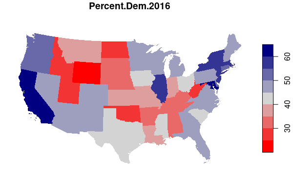
For example, maps of electoral results give a very different impression depending on whether you map by state or by county.
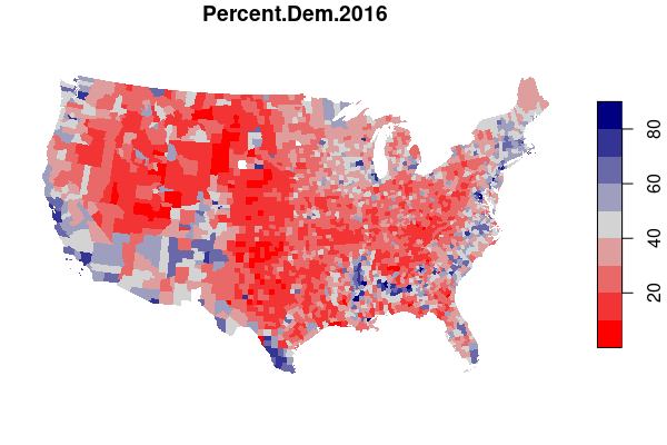
In drawing electoral boundaries, gerrymandering is an intentional political use of the MAUP where specific groups of voters are either "packed" into a small number of homogeneous districts or "cracked" across multiple districts in order to reduce the power and representation available to those groups.
There is no universally applicable solution to the MAUP. In cases where accuracy is not essential (such as with data exploration) or possible (such as with data that has been aggregated for privacy reasons), the uncertainty presented by the MAUP may be acceptable as long as caveats are provided along with the analysis. In other cases, more-sophisticated analytical approaches may be more appropriate.
Describing Area Patterns
Objects in space often tend to cluster together with other like objects. For example, wealthy neighborhoods are clusters of expensive houses and poor neighborhoods are clusters of more modest dwellings. Habitats can be more hospitable to different species of flora and fauna, and so different types of plants and animal species often live close together.
One of the primary ways of analyzing the spatial distribution of phenomenon is looking for geographical patterns of where points group together, or where high or low values are clustered together. Spatial autocorrelation is the clustering of similar values together in adjacent or nearby areas. One of the advantages of using geospatial data is that analysis of spatial autocorrelation can often provide insights into both the characteristics of different areas and the nature of the phenomenon being studied with the data.
Regional Descriptions
One way of describing patterns is by indicating what regions of have higher levels or a greater concentration of a phenomenon than other areas.
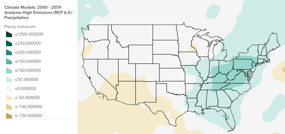
For example, the map below of projected annual precipitation changes in 2040-2059 based on the RCP 6.0 climate change scenario, the desert southwest region is modeled to see a reduction of up to 50 mm per year, while the Appalachian region in the northeastern part of the country is projected to be wetter, with 100 - 150 mm of precipitation above the historic average.
Core-Based Descriptions
Functional areas (core-based clusters) represent spatial correlation between a value and proximity to core areas.
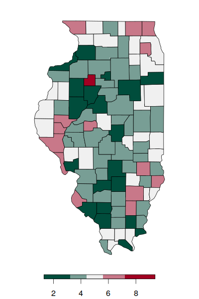
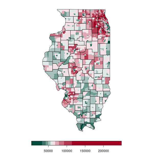
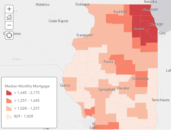
For example, in the State of Illinois, higher monthly homeowner mortgage costs tend to cluster in major urban areas. This variable exhibits strong autocorrelation with itself and strong correlation with proximity to urban cores (regional description).
Moran's I
While visible observation of spatial autocorrelation is useful when exploring data, more-rigorous means of quantifying autocorrelation are helpful when performing serious research.
The Moran's I statistic, developed by Patrick Alfred Pierce Moran (1950), quantifies spatial autocorrelation with values that vary from -1 (evenly dispersed = evenly spread out) to 0 (no autocorrelation) to +1 (completely clustered).
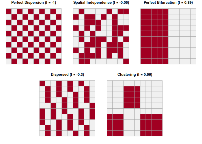
In a real-world Illinois example, clustering of median household income has high autocorrelation (I = 0.54), with high income counties largely clustered in a ring around Chicago, and low income counties clustered throughout the state.
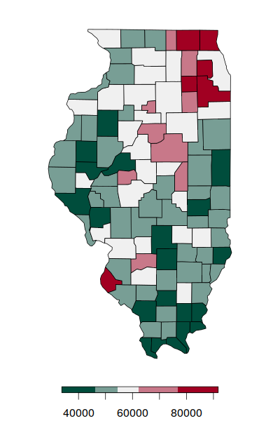
In contrast, the percentage of people who work at home exhibits no significant autocorrelation (I = 0.09) without either regular dispersion or regular clustering.
