Spatial Analysis of Crime Point Data in ArcGIS Pro
Revised 16 March 2026
Spatial analysis is the application of specialized statistical techniques to extract meaningful information from geospatial data. Those methods can be quite complex, but the fundamental ideas behind the methods are often conceptually straightforward, and the implementation of the algorithms in software means that most GIS users only need to have a general understanding of the capabilities and limitations of these methods in order to be able to use them effectively.
This module demonstrate some spatial analysis methods that can be used with point data in ArcGIS Pro. While this tutorial uses Chicago crime data as an example, these techniques can be applicable to any data consisting of points for a single type of phenomenon.
All videos on this page are silent.
- Crime Data Limitations
- Acquire and Process the Data
- Analyze the Data
- ModelBuilder Quirks
- Crime and Social Variables
- Dashboard
- Infographic
Crime Data Limitations
Some major cities make georeferenced crime location data available for analysis through their open data portals. This data has a number of limitations that you should be aware of as you perform your analysis:
- Data Recording Errors: This information is often based upon preliminary information supplied by the reporting parties that have not been verified, are subject to change, and may be corrupted by mechanical or human error.
- Classification Problems: Preliminary crime classifications may be changed at a later date based upon additional investigation. Some crime classification are ambiguous or overly broad. For example, burglary encompasses both residential and commercial, but the groups performing those crimes are different and different strategies are needed for addressing those two different types of crime.
- Anonymization: In order to protect the privacy of crime victims, addresses are shown at the block level only and specific locations are not identified. Accordingly, your analysis will need to be at a broad enough scale that this intentional spatial inaccuracy will not be a major factor.
- Geocoding Errors: As with all locations geocoded from place names, geocoding errors may give latitudes and longitudes that are not at the specified location. In some cases, these errors are obvious, such as when the points are at locations outside the police department's jurisdiction, or when coordinates are missing completely. However, an unknown number of points may also be placed at wrong locations. Most of these techniques work with large groups of points, so the effects of individual geocoding errors should be minimized.
- Temporal Errors: The dates and times in the data may not reflect the actual incident time, especially with types of crime (like domestic abuse) that occur over periods of time. Accordingly, comparisons over time may be skewed one way or the other.
- Underreporting: While records of highly-visible crimes like murder and arson are fairly complete, more than half of violent crimes in general and three-quarters of rapes are not reported to police ( Bureau of Justice Statistics 2012; RAINN 2018). In neighborhoods with poor community/police relations, victims may be less inclined to report crime to the police. Accordingly, analysis based on incident data from police departments will be incomplete for some crimes.
Acquire and Process the Data
Crime Data
The Chicago Police Department (CPD) provides a dataset of reported incidents of crime (with the exception of murders where data exists for each victim) that occurred in the City of Chicago since 2001. This dataset is made available through a dashboard and web map for convenient online analysis, and is also made available as raw CSV point data that can be imported into GIS. The original source of the data is the Chicago Police Department's CLEAR (Citizen Law Enforcement Analysis and Reporting) system.
The Chicago data portal uses the Socrata web app, which permits download of the data as CSV files with columns of latitude and longitude.
The app also provides a facility for filtering data. Because this data a variety of crimes over more than 20 years, downloading the millions of points and 1.6 gigabytes of data will result in data that will be very slow to analyze with ArcGIS Pro.
Therefore, in this example, we use filters to download separate Robbery data files for the years of 2019 and 2023.
Point data in CSV files with longitudes and latitudes can be imported into ArcGIS Pro and stored in the project database.
- Download a CSV file of crime data from the Chicago Data Portal.
- Search for Crime and select the Crimes - 2001 to Present data set.
- Under Actions, Query Data.
- Apply filters for Primary Type (Robbery) and Year (2019).
- Export to CSV with a meaningful file name (Crime_2019).
- Repeat for a later period (2023) and save to a separate file (Crime_2023).
- Create a new project and a new map.
- Under Analysis, Tools, open the XY Table To Point tool to import the points into the project geodatabase.
- Input Table: browse on your local machine to find the CSV of crime points that you downloaded (Crime_2019).
- Output Feature Class: Give a meaningful name with no spaces or punctuation (Crime_2019).
- X Field and Y Field: Make sure these are automatically set to the Latitude and Longitude columns.
- Repeat with the 2023 data.
- Symbolize with semitransparent hollow circles (80% transparency and multiply blending) so you can see point clusters.
Viewing Attributes
View the Attribute Table to find the count of features and the different available attributes.
You can get statistical summaries of columns (including the count of crimes) by clicking on a column and selecting Explore Statistics.
Neighborhood Areas
While neighborhoods are vernacular areas that often have unclear and contested boundaries, cities commonly create data files for neighborhoods that define unofficial boundaries that are useful for reference and context.
Note that neighborhoods are used in this tutorial for aggregating crime points rather than census tracts because the larger neighborhood areas mitigate the small numbers problem that would be more common with smaller tract areas and often sparse crime location data.
The City of Chicago makes neighborhood boundaries available as shapefiles that can be downloaded, unzipped, and imported into ArcGIS Pro.
- Download the zipped shapefile of neighborhood boundaries from the Chicago Data Portal.
- Use the Windows Explorer to extract the contents of the .zip file so they are visible to ArcGIS Pro.
- Under Analysis, Tools open the Export Features tool to import the boundaries into the project geodatabase.
- Input Features: Navigate to the .shp file.
- Output Features: Navigate to the project geodatabase and specify a new feature class name (Neighborhoods)
Census Tracts
For this example, we get demographic data for census tracts from the the US Census Bureau's 2019-2023 American Community Survey five year estimates.
Census tracts are organizational boundaries used for USCB data collection that are drawn to roughly align with neighborhood borders and, ideally, contain 4,000 residents, although the number of residents can vary depending on local characteristics (USCB 2019).
For convenience, we will use the tracts layer from the Minn 2019-2023 ACS feature service from the University of Illinois ArcGIS online organization.
- Under Analysis, Tools open the Export Features tool to import the boundaries into the project geodatabase.
- Input Features: Under ArcGIS Online, find the Minn 2019-2023 ACS feature service and navigate to the Tracts layer.
- Output Feature Class: Navigate to a new name in your project geodatabase (Census_Tracts)
- Expression: Add a filter to import only tracts in Cook County (GEOIDFQ begins with '1400000US17031'). See this tutorial for more information on GEOIDFQ and FIPS codes.
- Symbolize by the desired attribute (Median HH Income).
Analyze the Data
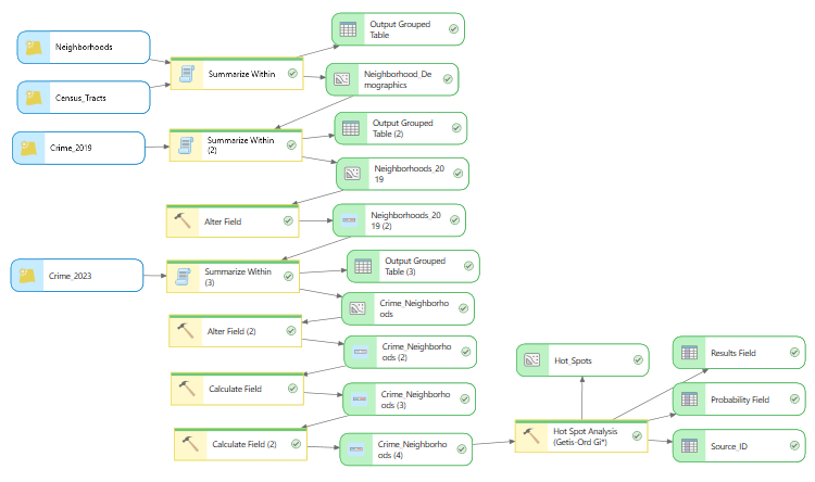
ModelBuilder
ModelBuilder is a visual programming language in ArcGIS Pro that allows you use a graphical editor to create custom tools that allow you to automate complex, tedious, or repetitive tasks where there are consistent step-by-step workflow sequences of operations.
Using ModelBuilder, you graphically chain together sequences of tools from the toolbox. This will be useful for this example because you will be executing a long sequence of tools, and using them in a ModelBuilder diagram will both make it easier to keep track of what you are doing and will allow you to easily rerun the analysis if you need to modify or fix one step in the analysis.
To start a new ModelBuilder diagram, on the Analysis ribbon, select ModelBuilder.
Save ModelBuilder
You should periodically save your ModelBuilder diagrams from the ModelBuilder ribbon as you work on your project.
- Regular model saving will mitigate loss of work if the software crashes.
- Note that the ModelBuilder Save button is separate from the Save Project button at the top of the screen for the project as a whole.
- Make sure to Save the ModelBuilder diagram before exporting a project package, or your changes may not be saved in the package.
Neighborhood Demographics
Demographics are "the statistical characteristics of human populations (such as age or income)" (Merriam-Webster 2024).
To analyze the relationship of crime to community characteristics, we need demographic data for the neighborhoods.
The neighborhood data from the City of Chicago contains only boundaries, so we will have to use a spatial join to summarize census tract demographics within neighborhoods.
A spatial join is a join where data from a join data set is copied into a target data set based on proximity of features in the two data sets.
Add the Summarize Within tool to your diagram.
- Input Polygons: Neighborhoods
- Input Summary Features: Census_Tracts
- Output Feature Class: Neighborhood_Demographics
- Keep all input polygons: Leave checked
- Add shape summary attributes: Deselect because we don't need counts of tracts.
- Summary Fields: Add fields that will be transferred from the tract data along with how the software should handle multiple join features (tracts) within a single target feature (neighborhood)
- Total Population (sum)
- Median Household Income (mean)
- Median Age (mean)
- Percent Foreign Born (mean)
- Add another Summarize Within tool to your diagram to perform a spatial join to get neighborhood crime counts for 2019.
- Input Polygons: Neighborhood_Demographics
- Input Summary Features: Crime_2019
- Output Feature Class: Neighborhoods_2019
- Keep all input polygons: Leave checked
- Add the Alter Field tool to rename the new count.
- Input Table: Neighborhoods_2019
- Field Name: Count of Points
- New Field Name: Count_2019
- New Field Alias: Count_2019
- Add a second Summarize Within tool to your diagram to perform a spatial join to get neighborhood crime counts for 2023.
- Input Polygons: Neighborhoods_2019
- Input Summary Features: Crime_2023
- Output Feature Class: Crime_Neighborhoods
- Keep all input polygons: Leave checked
- Add a second Alter Field tool to rename the new count.
- Input Table: Crime_Neighborhoods
- Field Name: Count of Points
- New Field Name: Count_2023
- New Field Alias: Count_2023
- Add to Display and symbolize by the new fields to verify the summarization worked.
- You can view the attribute table and sort by the crime count column to see the neighborhoods with the lowest and highest counts. If you select a row, it will be highlighted on the map.
- Input Table: Crime_Neighborhoods
- Field Type: Double (change this before adding the new name)
- Field Name: Rate_2023
- Expression: Divide Count_2023 by Total_Population and multiply by 1000 to get the rate per 1k.
- Input Table: Crime_Neighborhoods
- Field Type: Double (change this before adding the new name)
- Field Name: Percent_Change
- Expression: Divide Count_2023 by Count_2019, subtract one, and multiply by 100 to get percent change. Add 0.1 to the 2019 count to avoid a divide by zero problem in neighborhoods where there were zero reported incidents in 2019.
- Unusual events (like an isolated mass shooting) can result in random spikes in low population areas (the small numbers problem).
- Displacement of locations for anonymization to protect victims can cause individual area numbers to be artificially low or high.
- Aggregation by area is subject to the modifiable areal unit problem (MAUP) since using a different set of areas that are larger, smaller, or have different boundaries can result in significantly different results.
- To be a statistically significant hot spot, a feature will have a high value and be surrounded by other features with high values as well.
- The local sum for a feature and its neighbors is compared proportionally to the sum of all features.
- When the local sum is very different from the expected local sum, and when that difference is too large to be the result of random chance, a statistically significant z-score results.
- Use of this tool will help you assess whether the patterns you see in your data are the result of real spatial processes at work or just the result of random chance.
- Input Feature Class: Crime_Neighborhoods
- Input Field: Rate_2023
- Output Feature Class: Hot_Spots
- The resulting layer is colored red for hot spots where there are statistically significant clusters of higher levels of crime. The areas are colored blue for cold spots where there are statistically significant clusters of low levels of crime.
- Poverty: Poorer places tend to have higher crime
- Mixed land use: Places that have a mix of residential and commercial activity have higher levels of crime
- Population density: Places where people live very close together tend to have fewer people watching out for each other
- Residential turnover: In places where people are constantly moving in and out, it is more difficult to know who is an intruder
- Family instability: Neighborhoods with higher rates of divorce, separation, and single-parent households have lower levels of formal and informal social control.
- Pop per Square Mile (population density)
- Median Household Income (poverty)
- % Vacant Units (neighborhood stability)
- % Single Mothers (family instability)
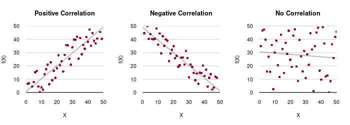
- If there is correlation, the points in an X/Y scatter chart will form something like a diagonal line upwards (positive) or downwards (negative) across the chart.
- If there is no correlation, the points will be erratically distributed around the chart area.
- The range of R-squared is from 0.000 (no fit) to 1.000 (perfect fit).
- Values of less than 0.100 can usually be considered to represent no meaningful relationship.
- In the social sciences where relationships often involve the complex interplay of ambiguous factors, values as low as the 0.100 to 0.300 range can be considered strong enough to merit further investigation.
- In the natural sciences, values above 0.700 are often expected to consider a model to have a strong fit.
- Select the layer you want to analyze in the Contents pane and then select Data, Visualize, Create Chart, Scatter Plot.
- Set the X and Y variables to examine correlations.
- Using a log scale can be useful when the values are skewed to the low end of the distribution.
- If desired, you can add the chart to a layout.
- Right click on your Crime_Neighborhoods layer in Contents and select Sharing and Share as Web Layer.
- Provide a meaningful name (Minn_2023_Chicago_Robbery).
- Provide a summary.
- Share with Everyone.
- Analyze to make sure everything is OK.
- If you get an error that, Unique numeric IDs are not assigned, click on the ellipsis (...) on the message and select Auto-Assign IDs Sequentially.
- After the layer is published, go to your ArcGIS Online Content page and open the layer in a new map.
- Change the variable to a categorized rate (Rate_2023) and rename it.
- Add neighborhood labels without halos.
- Configure the popups to display only meaningful values.
- In the layer properties, Group to create a group layer and rename it (Robbery in Chicago). On small screens you may need to scroll down in the properties list.
- In the group layer properties under Visibility, turn on Exclusive visibility so the different map layers can only be displayed one at a time.
- In the group layer properties, change blending to Multiply.
- Duplicate the rate layer and change the variable to the categorized change (Percent_Change) and rename it
- Duplicate the layer and change the variable to the categorized count (Count_2023). Counts should be displayed as bubbles (counts and amounts (size) with an outline) because choropleths of counts in areas with different sizes can give a distorted perception of where high or low counts are located.
- Save the map under a meaningful name (Minn 2023 Chicago Robbery).
- Share the map with Everyone.
- On your portal Content page, Create app with Experience Builder.
- Start with a Blank grid template.
- Rename the app.
- Add a Map widget, Select map, and Add new data with the web map you created above.
- Under Tools turn on the Layers selector.
- Save your changes.
- Add a Chart widget of type Column chart.
- Content, Data, Select Data with the map and the variable showing change in crime rates by neighborhood (Rate_2023).
- Chart type: Column chart
- Category type: By group
- Category field: pri_neigh
- Statistics: No aggregation
- Number fields: Rate_2023
- Sort by: Value
- Under General remove the title to conserve vertical space.
- Under Axis add a Y-axis label so it is clear what the chart shows (Robberies per 1k).
- Repeat with a second chart for the percent change by neighborhood (Change_2023).
- Save the app.
- Add a Chart widget.
- Content, Data, Select Data with the map variable.
- Chart type: Scatter plot
- Data, X-axis number: Rate_2023
- Y-axis number: Median_Household_Income
- Under General remove the title to conserve vertical space.
- Under Axis add X- and Y-axis labels so it is clear what the chart shows.
- Save the app.
- Select the Page and add a Header.
- Add the Text (Robbery in Chicago, 2023).
- Remove the Menu since this is a single map app.
- Add a logo Image and fit, if desired.
- Change the Height to 70px to fit on small screens.
- Configure the main map Action and Add a trigger for Extent changes. This will trigger the dashboard graphics to show data only for the neighborhoods visible as the user zooms in and out.
- Select the Framework and Filter data records.
- For Action data, Select data for all three displayed variable.
- Save frequently. Actions sometimes cause the app to lock up.
- Select Live View to verify the map behaves as desired.
- Lock layout so the widget sizes and locations are fixed.
- Change share settings to Everyone.
- Preview to confirm the app functions as desired.
- Publish the app.
- Get the Published item link to distribute to viewers.
- Manually run the Export Features tool with the crime points for 2023.
- Input Features: Crime_2023
- Output Feature Class: Point_Snapshot (in the project geodatabase)
- Manually run the Export Features tool with the combined neighborhood analysis.
- Input Features: Crime_Neighborhoods
- Output Feature Class: Neighborhood_Snapshot (in the project geodatabase)
- Manually run Export Features tool with the ModelBuilder hot spot layer, which willpreserve the hot spot symbology and legend labeling.
- Input Features: ModelBuilder\Hot_Spots:Hot_Spots
- Output Feature Class: Hot_Spots_Snapshot (in the project geodatabase)
- Refresh the view of the database in the Catalog Pane to confirm the feature classes have been created.
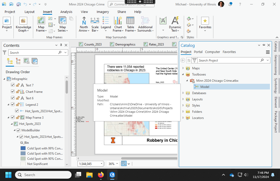
- Insert a Layout tabloid sized 11" x 17" in landscape orientation
- Properties, General rename the layout to Infographic.
- Add rectangles as neat lines.
- Frame line: 15 x 8 @ 1 x 2
- Logo: 2 x 1 @ 1 x 1
- Title: 10 x 1 @ 3 x 1
- Credits: 3 x 1 @ 13 x 1
- Insert a Picture of the logo.
- Add Straight text for the title (Robbery in Chicago, 2023)
- Add a Rectangle text box for the credits:
- Cartographer: Your Name
- Date: Current date
- Source: City of Chicago
- Create the crime points map.
- Insert a new map and give it an internal name of Crime_2023.
- Find your Points_Snapshot feature class in the Catalog Pane and drag it onto the new map.
- Change the Symbology for your points to 8 point, 80% transparent hollow dots that will make it possible to distinguish areas of high and low density.
- If needed, under Properties modify the map Coordinate System to use a cartographically appropriate projection (Web Mercator).
- Add the map as a map frame: 5 x 7 @ 1 x 2
- Hide the base map service credits.
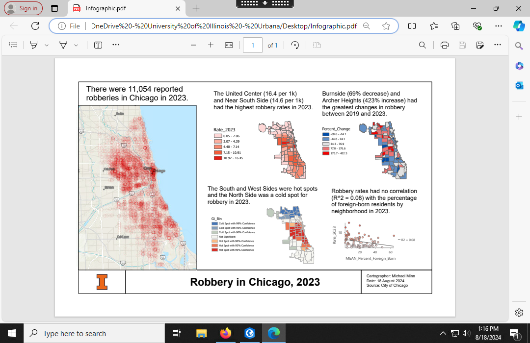
- Add a Straight text for the caption (There were 11,054 reported robberies in Chicago in 2023)
- Use 18 point Arial font to be consistent across the layout.
Crime Counts
Spatial joins can also be used to count the number of points within polygons. In this step, we use a spatial join to get counts of crime points within neighborhoods.
Crime Rates
Neighborhoods vary by population, and places with more people could be expected to have more crime, so maps of crime counts often become just maps of population that obscure where crime is actually a more serious problem.
Normalization is the adjustment of variable values to a common scale so they are comparable across space and time (Wikipedia 2023).
In this example we normalize crime counts by dividing by population to get crime rates that are comparable across different areas.
The small numbers problem occurs when small changes in counts create exceptionally high changes in rates when the population or incidence counts are small (Taklar et al. 2009). In this case, because the numbers of reported robberies per neighborhood is often small (there was one reported robbery in the Museum Campus neighborhood), the small numbers problem can cause the results to overstate or understate the severity of the condition.
Add the Calculate Field tool to your diagram.
Be aware that when you are creating a new field, you need to set the Field Type before providing a new Field Name, or the Field Type will default to non-numeric text and you will be unable to create a quantitative map symbology.
Remove the old layer from the map, Add to Display the layer with the new attribute, and symbolize to check the value.
Crime Change
Changes in the density of crime over time can be useful for assessing the success of past interventions, and identifying emerging areas that may need attention in the future.
Since we have crime counts for two different years, we can map percentage change between those two periods.
Add the Calculate Field tool to your diagram.
Hot Spot Analysis
While the counts and rates displayed above by neighborhoods may be adequate for your needs, maps can be deceiving.
With data like this, it can be helpful to analyze areas in the context of their immediate neighbors and the area as a whole.
The Hot Spot Analysis tool calculates the Getis-Ord Gi* statistic (pronounced gee eye star) for each feature in the context of its neighbors and reports the results as z-scores and p-values to indicate the probability that an area is a hot spot or cold spot.
The use of calculated probabilities makes this tool more rigorously defensible in research than simple visual inspection of points.
Add the Hot Spot Analysis tool to your diagram.
View Python
Behind the scenes, ModelBuilder creates Python code that you can view.
On the ModelBuilder ribbon, click the Export options (green arrow) and select Send To Python Window to view or copy the code.
ModelBuilder Quirks
ModelBuilder has some quirks you may need to work around as you build your analysis diagram.
Map Layers Disappear
When you re-run a tool that creates a feature class, ModelBuilder will delete the feature class and create a new feature class with that same name.
If you have a map that used the old feature class as a layer, the layer will be deleted from the map. You need to uncheck and then re-check Add to Display on the file in ModelBuilder.
If the map does not reappear, check other maps since ModelBuilder will often only add to the map that was present when the diagram was created.
General Function Failure
The General Function Failure seems to occur if you share a project package without saving the diagram from the ModelBuilder ribbon with the Save button. Although the absence of a meaningful message is annoying, this check is helpful because it will assure that your diagram is included in your project package so it will be available if you reopen the project from the package.
In some cases you might also need to completely close and restart ArcGIS Pro, reopen the project, and try sharing the package again.
It may also be necessary to close the ModelBuilder diagram before sharing.
Reopen the Model
If you close the model window, you can reopen it from the Catalog Pane by expanding Toolboxes, right-clicking on the model, and selecting Edit.
Crime and Social Variables
While having a descriptive understanding of where crime has occurred is useful, often we want to gain some understanding of why it occurred where it occured (explanatory model), or be able to have some idea about where it could occur in the future (predictive model).
Spatial analysis provides a wide variety of techniques for relating variables to each other in order to build models. While, crime, like most social phenomena, is driven by complex chains of causation and elements of randomness, it is possible to build models that offer insights into these processes. The examples below are highly simplified and do not provide a particularly strong fit with crime, but they are provided to offer some insights into the types of modeling that you can do with GIS.
Social Disorganization Theory
Social disorganization theory is a social ecology theory that asserts that crime is the result of an "inability of a community structure to realize the common values of its residents and maintain effective social controls" (Lersch 2004, 46; Sampson and Groves 1989, 177). Social disorganization theory has its roots in research performed in the School of Sociology at the University of Chicago beginning in the 1920s, most notably by Robert Park, Ernest Burgess, Clifford Shaw, and Henry McKay. Accordingly, these ideas are often referred to as Chicago School ideas.
Although the complexity of human society makes analysis of social disorganization similarly complex, a handful of neighborhood characteristics are theorized to lead to breakdowns in formal and informal social controls, and tend to correlate with higher levels of crime in specific areas ( Lersch 2004, 50-53; 148; Sampson and Raudenbusch 1999; 2001):
Although the American Community Survey tract data used in this example does not contain variables that directly measure the social disorganization theory factors directly, it does contain potential proxy variables that can be assumed to correlate with those factors. Those variables include:
Bivariate Correlation Charts
Correlation is "a relation existing between phenomena or things or between mathematical or statistical variables which tend to vary, be associated, or occur together in a way not expected on the basis of chance alone" (Merriam-Webster 2020).
While correlation does not prove that one of the measured characteristics causes the other, correlation is a common exploratory data analysis technique used to identify relationships in geospatial data that are deserving of further investigation.
A quick way to look for correlation between variables is to use an x/y scatter chart that graphs one variable on the x-axis in relation to a second variable on the y-axis.
Evaluation of R-squared to determine whether correlation should be considered strong or not depends on the type of phenomena being studied (Gupta et al. 2024).
To create an x/y scatter chart:
As shown in the video, the R-squared values for all four variables are fairly low (0.13 or less) and the X/Y scatter charts show a spreading pattern (heteroskedacity) that indicates that high crime areas tend to be low income, but low crime areas can be both low and high income.
This is consistent with crime / adversity mismatch research that shows no consistent relationship between socioeconomic disadvantage and levels of violence (Manguel 2021).
Ground Truth
In 1982, George L. Kelling and James Q. Wilson published a highly influential article entitled Broken Windows: The police and neighborhood safety that asserted a connection between crime and disorder as typified by the physical care of a neighborhood. If a window on a building is broken and no one fixes it, that is a sign that the people in the neighborhood do not care about their community. This leads to a breakdown in the informal community controls that normally hold crime in check.
Further research has suggested that broken windows is a fallacious confusion of correlation with causation (Thacher 2004), and the policing practices that follow from broken windows theory (like "stop-and-frisk") have been vigorously critiqued as counterproductive and socially unjust. However, the theory does lead us to ask questions about the relationship between crime and the built environment, something more fully fleshed out in urban planning practices like crime prevention through environmental design (CPTED) (Jeffery 1971).
Google Street View allows you to take a virtual walking tour of a neighborhood, and street view can be used to assess whether analysis performed in GIS is consistent with the conditions on the ground (ground truth). Care should be used in such qualitative analysis to mitigate the effects of confirmation bias that can reinforce preconcieved notions and stereotypes rather than validate analysis.
You can copy coordinates from a map in ArcGIS Pro by right-clicking on the location in the map, selecting Copy Coordinates, and search for that location in Google Maps.
Dashboard
Dashboards are web-based graphical user interfaces that provide an at-a-glance interactive summary of related information (analytics) on a single topic or business process.
ArcGIS Experience Builder is a web app available through ArcGIS Online or Portal for ArcGIS that can be used to build interactive web applications based on geospatial data without writing code. This section demonstrates creation of a dashboard with the analysis above using ArcGIS Experience Builder.
Publish the Feature Service
Dashboards are commonly built around a single feature service that provides the data for the map and graphics.
Publishing a service is the process of making data available as a service from servers or cloud services like ArcGIS Online.
Feature services are services that allow you to access geospatial feature data across the internet from a geodatabase on a server.
For this dashboard we will publish the feature service from the Crime Neighborhoods feature class created above with the crime counts, demographic data, crime rates, and change over time by neighborhood.
Create the Map
Create the Experience
Add the Main Map Widget
Add a Legend Widget
Thematic maps need a legend so map users can understand what values are associated with the different symbol sizes or colors.
Add Column Charts
Add an X-Y Scatter Chart
Add a Header
Add Actions
Actions in Experience Builder cause changes in one widget to trigger changes to other widgets. One common action is changing the displayed values in charts based on the change of extent (zooming) in the main map.
Publish the App
Infographic
An Infographic clearly and succinctly presents a variety of information and visualizations on a single graphical layout. This section demonstrates how to create an infographic layout for crime data in ArcGIS Pro.
Export Feature Classes
Because feature classes created in ModelBuilder will be replaced if you modify or re-run the model, you should manually export snapshots of your ModelBuilder feature classes and use those snapshots for creating visualizations (below).
A snapshot of your feature classes should be exported to the project geodatabase to keep the analysis data together with the original source data.
Infographic Layout
Main Map
Small Maps
To create the infographic, we will need to place the different feature classes on separate maps.
- Create the rate map.
- Insert a new map and give it an internal name of Rates_2023.
- Find your Neighborhoods_Snapshot feature class in the Catalog Pane and drag it onto the new map.
- Symbolize by the Rate_2023 in the color palette of your choosing.
- Adjust the legend label precision to match the data accuracy.
- Hide the base map.
- If needed, under Properties modify the map Coordinate System to use a cartographically appropriate projection (Web Mercator).
- Create the change map.
- In the Catalog Pane, Duplicate the rate map and rename it to Change_2023.
- Symbolize by Percent_Change with a diverging color scheme to make it easier to distinguish areas where crime is increasing vs. decreasing.
- Adjust the legend label precision to match the data accuracy.
- Create the hot spot map.
- In the Catalog Pane, Duplicate the rate map and rename it to Hot_Spots.
- Symbolize the layer for hot spots.
Small Map Frames and Legends
Add the three small maps to the infographic as map frames with captions.
- Small map frames: 2.3 x 3
- Remove the border
- Add a legend
- Add caption text (18 pt Arial)
Correlation Results
Add a correlation x/y scatter chart to your Rate_2023 map with the crime rate on the y-axis and a derived demographic variable you think might be correlated with that rate on the x-axis (Percent_Foreign_Born).
Click on the rate map frame to make it the active map and add a chart frame for the scatter chart to your layout.