Weather Data Analysis in R
This tutorial covers the visualization and basic descriptive analysis of historic weather data in R.
R Libraries
The following R libraries will be used by code in this tutorial and you should install them if you haven't already.
install.packages("xts")
install.packages("tsbox")
install.packages("forecast")
Acquire the Data
The National Oceanic and Atmospheric Administration (NOAA) is a US federal government agency formed within the Commerce Department in 1970 by combining the U.S. Coast and Geodetic Survey (founded under President Jefferson in 1807 as the Survey of the Coast), the Weather Bureau (founded in 1870), and the US Commission of Fish and Fisheries (founded in 1871) (NOAA 2021).
NOAA's mission is, " To understand and predict changes in climate, weather, oceans, and coasts, to share that knowledge and information with others, and to conserve and manage coastal and marine ecosystems and resources" (NOAA 2021).
As part of that mission, NOAA makes a wide variety of earth observation data available to the public, including historical weather observations collected by NOAA's National Weather Service.
The video below shows how to download historical weather observation data from NOAA's Climate Data Online web portal.
- Under Select Weather Observation Type/Dataset, select Daily Summaries.
- Leave Select Date Range as the default because the available data will depend on which weather observation station you select on the next screen.
- Under Search For, leave the default of Stations.
- Under Enter a Search Term, enter the name of your county and state.
- When the map pops up, select More Search Options, select Air Temperature and Precipitation as well as a 20-year date range to the present.
- Run the search and click on station icons on the map to find a station that a Period of Record with adequate date coverage. Twenty years or more will be most useful for trend analysis. Airports are usually a safe bet.
- In the selected station, click, ADD TO CART.
- Click on the Cart in the top right corner
- On the Select Cart Options page, under Select the Output Format, choose Custom GHCN-Daily CSV.
- Under Select the Date Range, select the desired date range. Note that this dialog will limit you to the dates for which data is available for this particular station and will also limit you to 25 years. For trend analysis, you will likely want to select all available dates.
- Click CONTINUE to proceed to the Custom Options: Daily Summaries page.
- Under Station Detail & Data Flag Options, select Station Name and Geographic Location.
- Under Select data types for custom output choose the selected options. For this example, we use all Precipitation, Air Temperature, and Wind variables and CONTINUE.
- On the Review Order page, Enter e-mail address and SUBMIT ORDER.
- Wait for an e-mail with a link to your data.
- Download the linked CSV to your local drive.
Process the Data
Load the Data
Note that the default name for this file will be your order number and you should probably rename it to something more meaningful so you can keep track of which file is which.
You can load the .csv data file with the read.csv() function and list the available variables with the names() function.
csv = read.csv("2650569-daily-summary.csv", as.is=T)

names(csv)

	 [1] "STATION"   "NAME"      "LATITUDE"  "LONGITUDE" "ELEVATION" "DATE"
	 [7] "AWND"      "FMTM"      "PGTM"      "PRCP"      "SNOW"      "SNWD"
	[13] "TAVG"      "TMAX"      "TMIN"      "WDF2"      "WDF5"      "WSF2"
	[19] "WSF5"

range(csv$DATE)

	[1] "1997-06-01" "2021-07-10"
The variables of particular interest for this analysis are the following.
- TMAX: Maximum temperature in degrees Fahrenheit
- TMIN: Minimum temperature in degrees Fahrenheit
- PRCP: Precipitiation in inches
Convert to a Time Series
A time series is "a set of data collected sequentially usually at fixed intervals of time" (Merriam-Webster 2021). Time series data has characteristics that make it very useful for analyzing phenomenon that change over time.
There are a wide variety of different libraries and classes are available for manipulating and analyzing time series data in R, and deciding which one to you can be confusing (Hyndman 2021).
This tutorial will use the xts library, which provides an extension of the zoo and ts classes for representing time series data in R.
This tutorial will also use the tsbox library for conversion between time series representations in order to take advantage of capabilities in the different libraries.
- The xts() function creates a time series object. The order.by parameter uses the dates from the data, which are converted to R Date objects by the as.Date() function.
- The ts_regular() function gives the time series a regular (daily) interval by adding NA values for missing dates. A regular interval will be needed later for decomposition analysis.
- The na.fill() function fills in those missing dates by duplicitating (extending) values from previous days.
- The window() function clips off the starting and ending dates so the number of years covered is a multiple of four. This will be needed later when the data needs to be aggregated into monthly periods.
library(xts)
library(tsbox)

historical = xts(csv[,c("TMAX","TMIN","PRCP")], order.by=as.Date(csv$DATE))

historical = ts_regular(historical)

historical = na.fill(historical, "extend")

historical = window(historical, start=as.Date("2000-01-01"), end=as.Date("2020-12-31"))
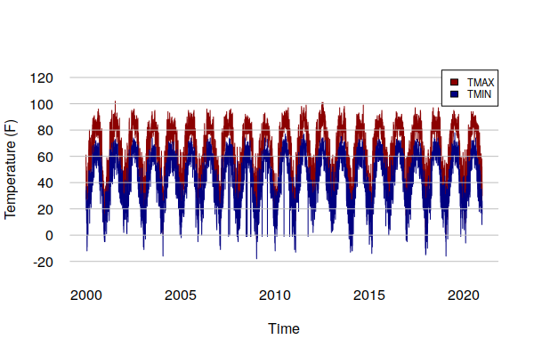
A plot() of TMIN and TMAX show the annual cycle of temperatures as well as extreme temperature events that spike above the general curve.
The ts_ts() function is used to plot ts objects rather than xts objects so that more control is available over the formatting of the charts.
plot(ts_ts(historical$TMAX), col="darkred", bty="n", las=1, fg=NA,
	ylim=c(-20, 120), ylab="Temperature (F)")

lines(ts_ts(historical$TMIN), col="navy")

grid(nx=NA, ny=NULL, lty=1, col="gray")

legend("topright", fill=c("darkred", "navy"), cex=0.7,
	legend=c("TMAX", "TMIN"), bg="white")
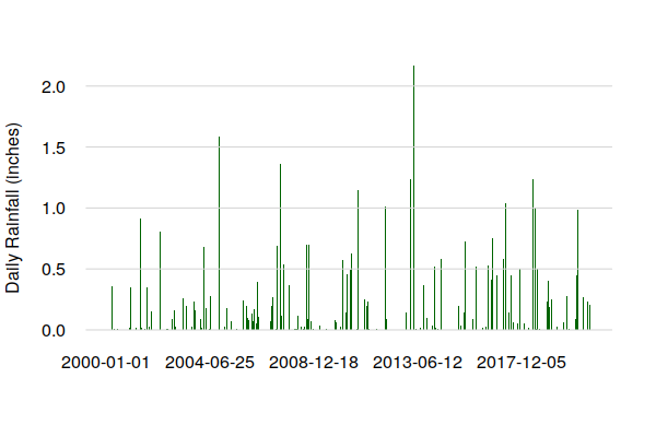
The plot() of daily precipitation shows no clear seasonal pattern, although the presence of a limited number of high precipitation days over the 23 years of this data is notable.
barplot(historical$PRCP, border=NA, col="darkgreen", ylim=c(0, 2),
	space=0, bty="n", las=1, fg=NA, ylab="Daily Rainfall (inches)")

grid(nx=NA, ny=NULL, lty=1)
Analyze the Data
Summary Descriptive Statistics
Running the summary() function will give basic descriptive statistics for the time series fields. You can subset the time series with logical conditions to find the dates for extreme conditions.
summary(historical)

	     Index                 TMAX             TMIN            PRCP
	 Min.   :2000-01-01   Min.   : -4.00   Min.   :-18.0   Min.   :0.00
	 1st Qu.:2005-04-01   1st Qu.: 45.00   1st Qu.: 28.0   1st Qu.:0.00
	 Median :2010-07-02   Median : 66.00   Median : 43.0   Median :0.00
	 Mean   :2010-07-02   Mean   : 62.69   Mean   : 41.9   Mean   :0.10
	 3rd Qu.:2015-10-01   3rd Qu.: 81.00   3rd Qu.: 58.0   3rd Qu.:0.03
	 Max.   :2020-12-31   Max.   :102.00   Max.   : 78.0   Max.   :3.76

historical[historical$TMIN == min(historical$TMIN)]

		   TMAX TMIN PRCP
	2009-01-16    9  -18    0

historical[historical$TMAX == max(historical$TMAX)]

		   TMAX TMIN PRCP
	2001-07-20  102   55 0.02

historical[historical$PRCP == max(historical$PRCP)]

		   TMAX TMIN PRCP
	2014-05-21   91   66 3.76
Seasonal Statistics
Time series representation also facilitates summary statistics of recurring periods, like months.
- The format() function with the %m format descriptor isolates the month portion of the date.
- The split() function breaks a vector into a data frame with separate fields based on a specific factor, in this case the month. The as.numeric() conversion is used to remove the time series date index so that dates are not included in the summaries.
- The sapply() function runs the summary() function on each field in the split data frame.
historical$MONTH = format(index(historical), "%m")

months = split(as.numeric(historical$TMAX), historical$MONTH)

sapply(months, summary)

		       1        2        3        4       5        6        7        8
	Min.    -4.00000  4.00000 12.00000 33.00000 48.0000 56.00000  65.0000 63.00000
	1st Qu. 27.00000 30.00000 42.00000 57.00000 68.0000 79.00000  81.0000 80.00000
	Median  34.00000 36.00000 50.00000 65.00000 77.0000 83.00000  85.0000 83.00000
	Mean    34.26575 37.79798 51.47005 64.94524 75.3149 83.23571  84.5169 83.37327
	3rd Qu. 41.00000 45.75000 61.00000 74.00000 84.0000 88.00000  88.0000 87.00000
	Max.    67.00000 72.00000 86.00000 90.00000 97.0000 99.00000 102.0000 97.00000
		       9       10       11       12
	Min.    52.00000 40.00000 16.00000  2.00000
	1st Qu. 74.00000 57.00000 43.00000 31.00000
	Median  80.00000 66.00000 52.00000 38.00000
	Mean    79.56111 66.24424 51.85079 38.42089
	3rd Qu. 85.00000 75.00000 59.75000 47.00000
	Max.    99.00000 93.00000 81.00000 73.00000

months = split(as.numeric(historical$TMIN), historical$MONTH)

sapply(months, summary)

			1         2        3        4        5       6        7
	Min.    -18.00000 -14.00000 -9.00000 12.00000 -1.00000 -1.0000 -1.00000
	1st Qu.   8.00000  13.00000 25.00000 33.00000 46.00000 57.0000 60.00000
	Median   20.00000  21.50000 31.00000 41.00000 52.00000 62.0000 65.00000
	Mean     17.64286  20.26599 31.00998 40.89603 52.34562 61.3254 63.74731
	3rd Qu.  28.00000  29.00000 37.00000 48.00000 60.00000 66.5000 69.00000
	Max.     57.00000  52.00000 61.00000 65.00000 72.00000 74.0000 78.00000
		       8        9       10       11        12
	Min.    -1.00000 -1.00000 -1.00000 -1.00000 -10.00000
	1st Qu. 58.00000 49.00000 36.00000 26.00000  15.00000
	Median  63.00000 55.00000 42.00000 32.00000  24.00000
	Mean    61.76805 54.63095 42.88633 32.19048  22.87404
	3rd Qu. 66.00000 61.00000 49.00000 39.00000  31.00000
	Max.    75.00000 72.00000 68.00000 61.00000  58.00000
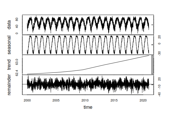
Time Series Decomposition
Time series decomposition separates a time series into three fundamental components that can be added together to create the original data:
- A seasonal component
- A long-term trend component
- A random component
When using historical data to anticipate what might happen in the future, we often wish to separates the seasonal and random components to see the long term historical trends.
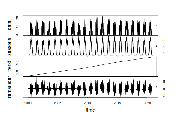
The stl() function performs this decomposition.
- The ts_ts() function from the library converts an xts field to a ts object that can be used with stl().
- The s.window parameter defines the smoothing to isolate the seasonal component (365 days = one year).
- The t.window parameter defines the smoothing to isolate the long-term trend (~20 years).
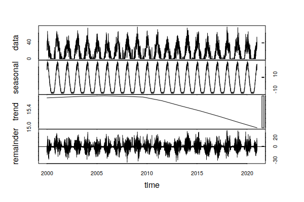
decomposition = stl(ts_ts(historical$TMAX), s.window=365, t.window=7001)

plot(decomposition)

summary(decomposition$time.series[,"trend"])

	   Min. 1st Qu.  Median    Mean 3rd Qu.    Max.
	  62.33   62.43   62.63   62.72   63.00   63.36
In this example, the trend indicates an increase of around one degree (F) in daily maximum temperatures over the period 2000 - 2020. In daily life, this is masked by seasonal swings (summer to winter) of around 45 degrees, and random daily variation of around 60 degrees.
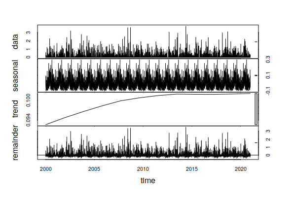
Performing the same analysis on daily precipitation, we also see an small trend in daily increase in precipitation of around 0.06 inches over the past 23 years, which translates to around one additional inch of rain per year (0.06 * 365 / 23).
decomposition = stl(ts_ts(historical$PRCP), s.window=365, t.window=7001)

plot(decomposition)

summary(decomposition$time.series[,"trend"])
Aggregation
Although having daily weather observations is extremely useful for analysis, direct visualization of daily observations relies on inexact (and occasionally deceptive) visual identification of patterns and trends. Visualization of decomposition captures trends, but can be confusing to folks with little or no exprience with time series analysis.
One common technique to address this issue with time series data is to aggregate values by months or years.
- With xts time series objects, the period.apply() function can be used to perform operations on blocks of observations across the time series. Those operations are specified with the FUN= parameter and commonly include min(), max(), and mean().
- period.apply() requires a regular (even) interval between periods. Because months are uneven, a seq() of regularly spaced index values is passed to the INDEX= parameter. The INDEX value is is a regular spacing that approximates 12 months per year when leap years are considered (365 + 365 + 365 + 366 / 48 = 30.4375).
- Because the periods need an even number of observations, the window() dates should be chosen so they encompass even multiples of four years to account for leap years.
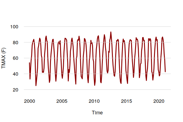
monthly.tmax = period.apply(historical$TMAX, INDEX = seq(1, nrow(historical) - 1, 30.4375), FUN = mean)

plot(ts_ts(monthly.tmax), col="darkred", ylim=c(20, 100),
	lwd=3, bty="n", las=1, fg=NA, ylab="TMAX (F)")

grid(nx=NA, ny=NULL, lty=1)
The aggregation by mean() smooths out the daily randomness to make the overall cycles and trends clearer.
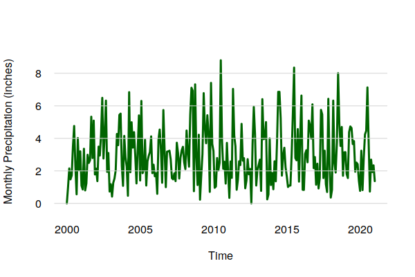
For precipitation, a sum() is more appropriate.
monthly.prcp = period.apply(historical$PRCP, INDEX = seq(1, nrow(historical) - 1, 30.4375), FUN = sum)

plot(ts_ts(monthly.prcp), col="darkgreen",
	lwd=3, bty="n", las=1, fg=NA, ylab="Monthly Precipitation (inches)")

grid(nx=NA, ny=NULL, lty=1)
The aggregation by mean() smooths out the daily randomness to make the overall cycles and trends clearer.
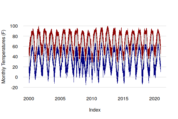
Area Plot
Area plots can be useful for showing extremes vs. averages with aggregated data. Averages smooth off the outliers, and with temperature data this can mask how hot or cold it can get in periods of extreme weather.
Area plots in base graphics can be drawn by creating polygons, although the process is cumbersome. The upper part of each polygon is one time series, and the lower part is the time series below it in reverse order using the rev() function.
tmax.mean = period.apply(historical$TMAX, INDEX = seq(1, nrow(historical) - 1, 30.4375), FUN = mean)
tmax.max = period.apply(historical$TMAX, INDEX = seq(1, nrow(historical) - 1, 30.4375), FUN = max)
tmin.mean = period.apply(historical$TMIN, INDEX = seq(1, nrow(historical) - 1, 30.4375), FUN = mean)
tmin.min = period.apply(historical$TMIN, INDEX = seq(1, nrow(historical) - 1, 30.4375), FUN = min)

tmax.area = c(as.numeric(tmax.max), rev(as.numeric(tmax.mean)))
tavg.area = c(as.numeric(tmax.mean), rev(as.numeric(tmin.mean)))
tmin.area = c(as.numeric(tmin.mean), rev(as.numeric(tmin.min)))

indices = c(index(ts_ts(tmax.mean)), rev(index(ts_ts(tmax.mean))))

plot(NA, xlim=range(indices), ylim=c(-20, 100),
	lwd=3, bty="n", las=1, fg=NA, ylab="Monthly Temperatures (F)")

polygon(indices, tmax.area, border=NA, col="darkred")
polygon(indices, tavg.area, border=NA, col="lightgray")
polygon(indices, tmin.area, border=NA, col="navy")

grid(nx=NA, ny=NULL, lty=1)
Holt-Winters Forecasts
Since time series analysis decomposes past weather observations into seasonal, trend, and random components, that data can be used to create forecasts based on an assumption that the observed patterns will continue into the future. This type of forecasting is especially useful in business for anticipating potential demand for seasonal products.
To forecast future temperatures based on historical observations, we can use Holt-Winters model that considers past seasonal cycles, trends, and random variation.
- We first create training data consisting of a time series of high temperatures aggregated by month. Monthly data is used instead of daily data because the hw() modeling function used in the next step will throw a "Frequency too high" error on daily data.
- The parameters to the hw() modeling function are the time series and the number of additional observations to forecast. h=60 indicates modeling five years into the future.
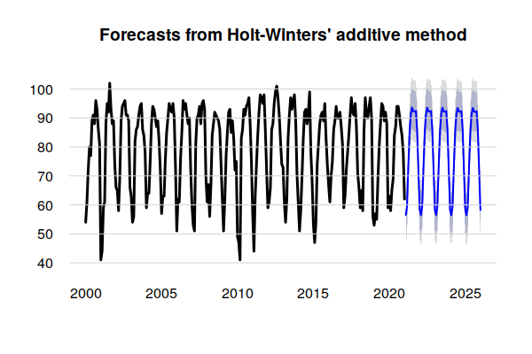
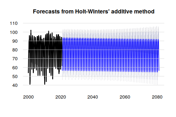
library(forecast)

training.data = period.apply(historical$TMAX, seq(1, nrow(historical) - 1, 30.4375), max)

model.tmax = hw(ts_ts(training.data), h=60)
A plot() of the model shows a forecast of future temperatures.
The dark blue line is the mean seasonal and trend components that are assumed to continue into the future in the same manner as in the past.
The gray lines above and below the seasonal trend represent a range of possible future values based on the random variation in the historical data. Given the amount of variation in the historical data and absence of a clear trend, the exponential smoothing methods used by the Holt-Winters model result in extreme peaks and wide uncertainty as the output extends far into the future.
plot(model.tmax, lwd=3, bty="n", las=1, fg=NA)

grid(nx=NA, ny=NULL, lty=1)
This forecasting method assumes the future will be like the recent past. Given the highly variable nature of both atmospheric and human processes, this may not be an reasonable assumption when projecting weather into the distant future.
This forecasting method does present an interesting way of discussing what the future could look like if those processes could be frozen in their current state. However, that should not be confused with a business-as-usual (BAU) scenario, since environmental processes are dynamic and continuing our current practices would still result in uncertain environmental changes.
model.tmax = hw(ts_ts(training.data), h=720)

plot(model.tmax, lwd=3, bty="n", las=1, fg=NA)

grid(nx=NA, ny=NULL, lty=1)
ARIMA Forecasts
The Holt-Winters modeling technique dates from the late 1950s, and although it is still applicable in a variety of situations (e.g. Mgale, Yan, and Timothy 2021), it is fundamentally a smoothing algorithm that seeks patterns by removing noise, rather than trying to understand the noise.
In contrast, auto regressive integrated moving average (ARIMA) modeling involves a more detailed analysis of the training data using lags and lagged forecast errors.
Accordingly, ARIMA can give much more detailed forecasts than Holt-Winters, although though this comes at a cost of being both more difficult to configure and more computationally intensive. For highly detailed data like weather observations, this can require hours of computing time rather than seconds.
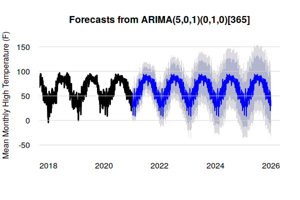
The first step is to use a function like auto.arima() to analyze the data and find appropriate model configuration parameters. Note that running auto.arima() on this 20-year daily data set may take around 50 minutes on a consumer-level PC.
training.data = ts_ts(historical$TMAX)

parameters = auto.arima(training.data)

print(parameters)

	ARIMA(5,0,1)(0,1,0)[365]

	Coefficients:
		 ar1      ar2     ar3      ar4     ar5      ma1
	      1.4871  -0.6970  0.1903  -0.0807  0.0377  -0.7694
	s.e.  0.0899   0.0672  0.0252   0.0210  0.0143   0.0896

	sigma^2 estimated as 113:  log likelihood=-27633.46
	AIC=55280.92   AICc=55280.94   BIC=55329.2
The parameters at the top of the model listing can be passed to the arima() function as the order and seasonal parameters to create a model for the forecast() function.
As with the Holt-Winters model above, the variability in the data contributes to extreme probability ranges that limit the utility of historically-based ARIMA forcasts with this type of data.
arima.model = arima(training.data, order = c(5,0,1), seasonal = list(order=c(0,1,0), period=365))

arima.tmax = forecast(arima.model, 1825)

plot(arima.tmax, lwd=3, bty="n", las=1, fg=NA,
	xlim=c(2018, 2026), ylab="Mean Monthly High Temperature (F)")

grid(nx=NA, ny=NULL, lty=1)
Heating and Cooling Degree Days
One consequence of the potential for higher temperatures is increased need for energy for building cooling and, conversely, decreased need for energy for building heating.
Two metrics for estimating the amount of energy used for building heating and cooling are heating degree days (HDD) and cooling degree days (CDD). These numbers represent the sum of the number of degrees for each day of the year where average temperatures are below 65 degrees (HDD) or above 65 degrees (CDD). At temperatures below 65 degrees, buildings need heating to keep occupants comfortable, and at temperatures above 65 degrees, buildings need cooling.
For example, if the average temperature on a particular day is 35 degrees, that day requires 65 - 35 = 30 HDD and no CDD. If the average temperature were 86 degrees, that day would require 86 - 65 = 21 CDD and no HDD.
CDD and HDD can also be seen as a proxy for discomfort, with higher CDD values in hotter climates and higher HDD values in cooler climates. However, discomfort is subjective as it also involves humidity, as well as personal physiology and preferences.
historical$TAVG = (historical$TMAX + historical$TMIN) / 2

historical$HDD = ifelse(historical$TAVG < 65, 65 - historical$TAVG, 0)

historical$CDD = ifelse(historical$TAVG > 65, historical$TAVG - 65, 0)
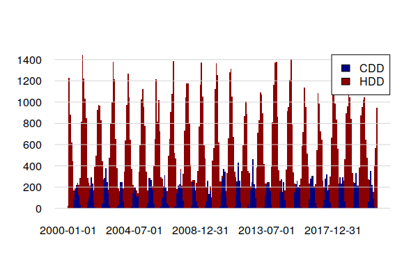
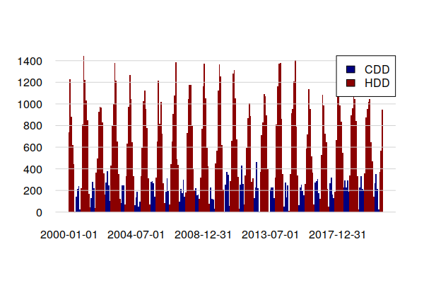
A barplot() shows CDD clumped in summers and HDD clumped in winters. In this cool climate, heating energy significantly outweighs cooling energy.
monthly.cdd = period.apply(historical$CDD, INDEX = seq(1, nrow(historical) - 1, 30.4375), FUN = sum)

monthly.hdd = period.apply(historical$HDD, INDEX = seq(1, nrow(historical) - 1, 30.4375), FUN = sum)

barplot(merge.xts(monthly.cdd, monthly.hdd),
	col=c("navy", "darkred"), las=1, fg="white",
	space=0, border=NA)

grid(nx=NA, ny=NULL, lty=1)

legend(x="topright", fill=c("navy", "darkred"), legend=c("CDD", "HDD"), bg="white")
Focusing on CDD, the time series decomposition shows a slight increasing trand over the 1998 - 2021 period, reflecting a slight increase in the number of days where air conditioning is needed.
decomposition = stl(ts_ts(historical$CDD), s.window=365, t.window=7001)

plot(decomposition)
In contrast, the trend over the 23 years of this historical data has been for HDD to drop. This hints that increases in energy for summer building cooling due to rising temperatures may be offset by decreases in winter building heating. However, because the technologies for heating and cooling are different (gas vs. electricity), this may presage need for increased investment in electrical power sources and distribution lines.
decomposition = stl(ts_ts(historical$HDD), s.window=365, t.window=7001)

plot(decomposition)
HDD and CDD can be estimated from monthly temperature averages.
historical$TAVG = (historical$TMAX + historical$TMIN) / 2

monthly.tavg = period.apply(historical$TAVG, INDEX = seq(1, nrow(historical) - 1, 30.4375), FUN = mean)

estimate.hdd = ifelse(monthly.tavg < 65, 65 - monthly.tavg, 0) * 30

estimate.cdd = ifelse(monthly.tavg > 65, monthly.tavg - 65, 0) * 30

barplot(merge.xts(estimate.cdd, estimate.hdd),
	col=c("navy", "darkred"), las=1, fg="white",
	space=0, border=NA)

grid(nx=NA, ny=NULL, lty=1)

legend(x="topright", fill=c("navy", "darkred"), legend=c("CDD", "HDD"), bg="white")
Extreme Precipitation Events
One of the anticipated challenges of anthropogenic climate change is the increase in extreme precipitation events that result in flooding (Denchak 2019).
The following code flags days with over (an arbitrarily chosen) one inch of precipitation, and aggregates them by year.
historical$FLOOD = ifelse(historical$PRCP > 1, 1, 0)

flooding = period.apply(historical$FLOOD, INDEX = seq(1, nrow(historical) - 1, 365.25), FUN = sum)

plot(ts_ts(flooding), col="darkgreen",
	lwd=3, bty="n", las=1, fg=NA,
	ylab="Annual Days with High Precipitation")

grid(nx=NA, ny=NULL, lty=1)

summary(as.numeric(flooding))

	   Min. 1st Qu.  Median    Mean 3rd Qu.    Max.
	  0.000   6.250   7.500   7.955   9.750  15.000
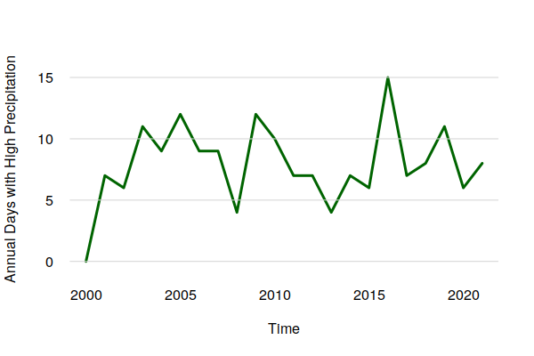
Despite what appears to be an upward trend in extreme precipitation days in the graph above, the time series decomposition points out that there was a drop over the 2000s that reversed in the 2010s. Accordingly, there is no clear evidence in this data of a long term increase in the normal days per year with extreme precipitation.
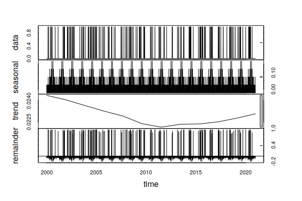
decomposition = stl(ts_ts(historical$FLOOD), s.window=365, t.window=7001)

plot(decomposition)
Saving Time Series Data
Because time series objects contain a variety of different interrelated components, they cannot be saved in simple files like .csv files.
However, you can save R objects to R data serialization (RDS) files so that you can reuse them in the future without having to go through the effort of running your processing code again.
saveRDS(historical, "2000-2020-historical.rds")
You can restore an objece with the readRDS() function.
historical = readRDS("2000-2020-historical.rds")