Summarizing Data in R (Descriptive Statistics)
This tutorial describes how to perform basic descriptive statistics using data frames in R.
Weather Data
The examples in this tutorial use historic weather data downloaded from the National Weather Service (NWS). The video below demonstrates how to download NWS data as well as comparable data from Weather Underground.
Importing Data Frames
You can import data into R from comma-separated variable (CSV) files.
It is important that the top row of your CSV file contain the names of your columns. Do not leave any blank rows at the top of your CSV file.
For this example, I assume I have a file of historic weather data named nws-spokane.csv. Use whatever name is appropriate as a string in the first parameter to the read.csv() function. This will read the contents of the file into the weather variable as a data frame. Type:
> weather = read.csv("nws-spokane.csv", as.is=T)
> weather
          DATE MAXTEMP MINTEMP AVGTEMP DEPARTURE HDD CDD PRECIPITATION SNOWNEW
1     1/1/2016      19       2    10.5     -16.8  54   0             0       0
2     1/2/2016      18       1     9.5     -17.9  55   0             T       T
3     1/3/2016      24       7    15.5     -12.1  49   0          0.09       1
4     1/4/2016      31      23    27.0      -0.7  38   0             T     0.4
5     1/5/2016      36      26    31.0       3.1  34   0          0.02       T
6     1/6/2016      36      32    34.0       5.9  31   0             T       T
7     1/7/2016      34      31    32.5       4.3  32   0             T       T
8     1/8/2016      34      29    31.5       3.1  33   0             T     0.3
9     1/9/2016      38      26    32.0       3.4  33   0             0       0
10   1/10/2016      30      27    28.5      -0.3  36   0             T       T
...
When you displayed the contents of the weather variable you probably got a long listing of the entire table. Since your console is not wide or tall enough to have space for all the data, it scrolled off the screen.
When looking at the content of large data on a console, you will generally need to select a subset of the data to view.
Data Frame Columns
Data frames are like spreadsheets. To see the column names, use the colname() function. Type:
> colnames(weather)
 [1] "DATE"          "MAXTEMP"       "MINTEMP"       "AVGTEMP"
 [5] "DEPARTURE"     "HDD"           "CDD"           "PRECIPITATION"
 [9] "SNOWNEW"       "SNOWDEPTH"
You can show the contents of a column in a data frame by giving the name of the data frame variable, a dollar sign, and the name of the column you want to see. To get the contents of the column Mean.TemperatureF, type:
> weather$Mean.TemperatureF
  [1] 10.5  9.5 15.5 27.0 31.0 34.0 32.5 31.5 32.0 28.5 26.5 32.5 35.0 29.5 24.5
 [16] 32.0 35.0 34.5 34.0 36.0 35.0 40.0 37.0 32.5 31.0 36.0 40.0 39.0 33.5 32.5
 [31] 31.5 30.0 27.5 26.0 32.0 39.5 37.5 33.0 39.0 40.0 35.5 37.0 44.5 40.0 42.5
 [46] 49.0 48.0 45.0 41.5 41.0 37.0 34.5 36.0 34.5 39.0 42.0 43.5 47.0 44.5 40.0
 [61] 39.5 43.5 44.5 45.5 48.5 43.5 40.0 37.5 39.5 43.0 42.0 42.5 40.0 39.5 38.0
 [76] 39.0 39.0 39.0 44.5 50.5 48.5 38.5 42.0 44.5 42.0 42.0 42.5 39.0 44.0 49.5
 [91] 51.5 55.0 56.5 52.5 46.0 43.5 50.0 57.0 63.0 61.0 57.0 55.5 53.5 48.5 46.0
[106] 44.5 50.0 56.5 63.0 63.0 67.5 68.0 64.0 56.0 51.0 47.5 50.5 54.5 55.5 49.5
[121] 55.0 58.0 64.5 66.5 64.5 63.0 65.0 67.5 64.5 49.5 54.0 58.0 62.0 60.0 60.0
...
Basic Descriptive Statistics
The following R functions can be useful for basic statistical analysis of vectors of data:
- max() the maximum value in a vector
- min() is the minimum value in a vector
- mean() is the mean (average) value of the values in a vector
- sd() is the standard deviation of the values in a vector
- length() is the number of values in a vector
You can use whole columns as vector parameters to functions. Type:
> max(weather$MAXTEMP)
[1] 97
> min(weather$MINTEMP)
[1] -7
> mean(weather$AVGTEMP)
[1] 50.45082
> sd(weather$AVGTEMP)
[1] 15.81478
> length(weather$AVGTEMP)
[1] 366
If your data has missing elements, these are represented as "NA." Many statistical functions consider vectors containing NA to be incomplete and return NA. If this happens, you need to tell the function to remove NA values with the na.rm=T parameter:
> mean(weather$AVGTEMP, na.rm=T)
[1] 50.45082
Subsets of Data Frames
The data in data frames can be accessed like a spreadsheet or array using square brackets: variable[row, column]. For example, to access row number 5 and column number 3 (the mean temperature in my data), type:
> weather[5, 3]
[1] 26
You can leave one of the dimensions blank in bracket notation to access all columns from a single row or all rows from a single column. To show all values from row 5, type:
> weather[5,]
      DATE MAXTEMP MINTEMP AVGTEMP DEPARTURE HDD CDD PRECIPITATION SNOWNEW
5 1/5/2016      36      26      31       3.1  34   0          0.02       T
  SNOWDEPTH
5         9
You can display a range of rows using a numeric range. Type:
> weather[1:3,]
      DATE MAXTEMP MINTEMP AVGTEMP DEPARTURE HDD CDD PRECIPITATION SNOWNEW
1 1/1/2016      19       2    10.5     -16.8  54   0             0       0
2 1/2/2016      18       1     9.5     -17.9  55   0             T       T
3 1/3/2016      24       7    15.5     -12.1  49   0          0.09       1
  SNOWDEPTH
1         9
2         8
3         8
You can also use bracket notation with condition statements to select rows from the data frame. For example, to select the rows for days where the temperature never got above freezing:
> freezing = weather[weather$MAXTEMP <= 32,]
> freezing
          DATE MAXTEMP MINTEMP AVGTEMP DEPARTURE HDD CDD PRECIPITATION SNOWNEW
1     1/1/2016      19       2    10.5     -16.8  54   0             0       0
2     1/2/2016      18       1     9.5     -17.9  55   0             T       T
3     1/3/2016      24       7    15.5     -12.1  49   0          0.09       1
4     1/4/2016      31      23    27.0      -0.7  38   0             T     0.4
10   1/10/2016      30      27    28.5      -0.3  36   0             T       T
11   1/11/2016      31      22    26.5      -2.4  38   0          0.02     0.2
15   1/15/2016      31      18    24.5      -5.1  40   0          0.02     0.5
33    2/2/2016      32      23    27.5      -4.0  37   0             0       0
34    2/3/2016      32      20    26.0      -5.5  39   0          0.11     1.1
340  12/5/2016      31      20    25.5      -3.3  39   0             T       T
...
To get just the number of rows (i.e. the number of days), use the nrow() function. Type:
> nrow(freezing)
[1] 29
Line Charts
The plot() function is a generic graphing function that displays different types of graphs depending on what type of data you give it as parameters. To show a time series of mean temperature, type:
> plot(weather$AVGTEMP)
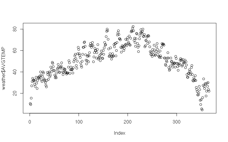
By default, plot of a vector plots dots. If you want to plot lines, you need to set the parameter type="l" for line graph. plot(), like many R functions has many different parameters, although there are default values for parameters that you do not provide. Unlike Excel, parameters to R functions can be in any order as long as you give a name:
> plot(weather$AVGTEMP, type="l")

Note that at the console, you can use the up and down arrow keys to scroll through the commands you have typed previously.
To get meaningful labels on the X axis you need to give as set of X values to go with the Y values (the temperatures) that are being plotted. X values must be numeric, but since the dates in the CSV file are strings, the as.Date() function must be used to convert them to numbers that can be plotted.
> weather$DATE = as.Date(weather$DATE, format="%m/%d/%Y")
You can then specify the x and y values for the plot():
> plot(x = weather$DATE, y = weather$AVGTEMP, type="l")
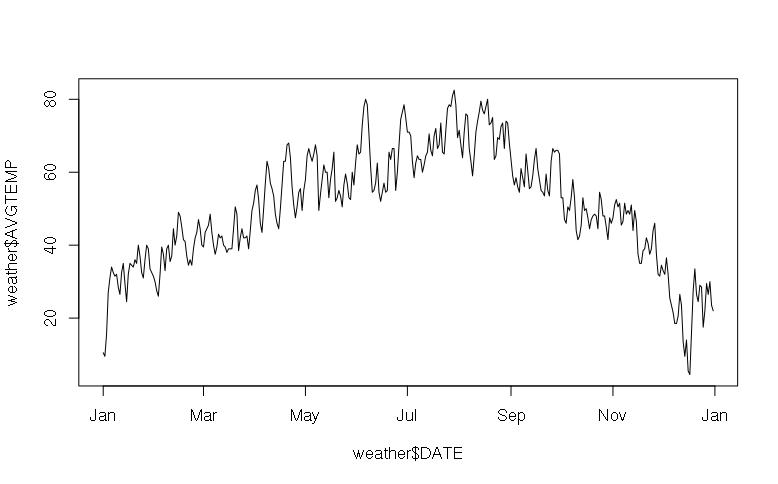
If you want to plot in another color other than black, you can give another color in the col parameter. This parameter accepts common names as strings (e.g. red, blue, green, brown, etc.) as well as a number of custom names (see the table here) or, if you know CSS color notation, as #RRGGBB. Type:
> plot(x = weather$DATE, y = weather$AVGTEMP, type="l", col="darkgreen")
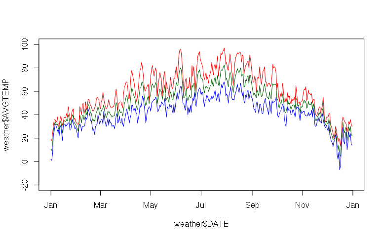
If you want to add additional lines to a plot, you can use the lines() function with parameters similar to plot(). Type:
> lines(x = weather$DATE, y = weather$MAXTEMP, col="red")
> lines(x = weather$DATE, y = weather$MINTEMP, col="blue")
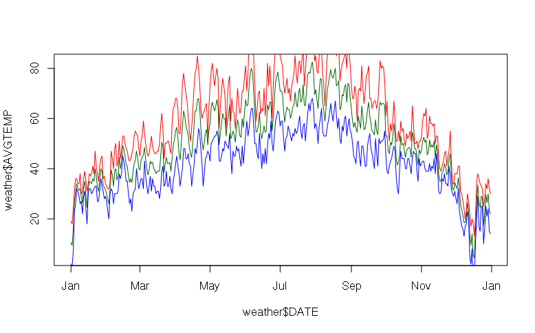
plot() chooses the range of Y values based on the first line plotted. If your additional lines extend above and/or below the plot, you need to use a ylim parameter on your initial plot. This parameter is a two-element vector: the first element is the low value for the Y axis and the second element is the high value. For example, to have the y-axis extend from -50 degrees to 100 degrees, type:
> plot(x = weather$DATE, y = weather$AVGTEMP, type="l", col="darkgreen", ylim=c(-20, 100))
> lines(x = weather$DATE, y = weather$MAXTEMP, col="red")
> lines(x = weather$DATE, y = weather$MINTEMP, col="blue")
Smoothing Lines
With data like temperatures where there is alot of individual variation, it can be difficult to see the overall trend.
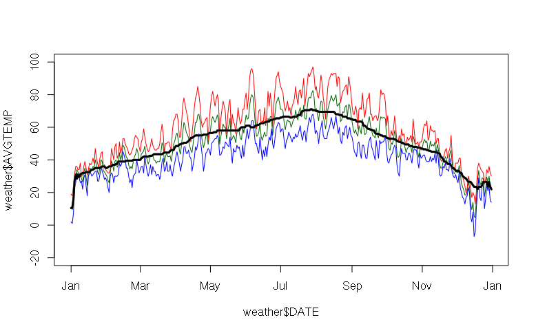
There are a variety of methods for smoothing lines. One quick technique is the running median that progressively moves a window across the values and takes the median of all values in the window.
Wider windows create smoother lines.
For example, when using the runmed() function to run a 61-day moving window across the mean temperature data, the sine wave of temperature across the year starts to become apparent:
> plot(x = weather$DATE, y = weather$AVGTEMP, type="l", col="darkgreen", ylim=c(-20, 100))
> lines(x = weather$DATE, y = weather$MAXTEMP, col="red")
> lines(x = weather$DATE, y = weather$MINTEMP, col="blue")
> smooth = runmed(weather$AVGTEMP, 61)
> lines(x = weather$DATE, y = smooth, col="black", lwd=3)
Histograms
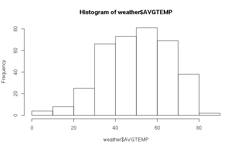
R has a native histogram function hist() that can be used to show the distribution of values in a vector:
> hist(x = weather$AVGTEMP)
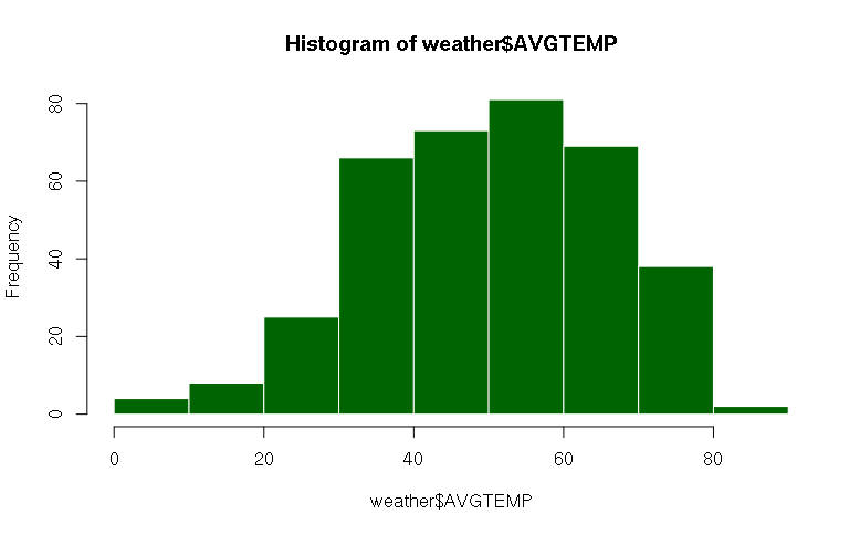
To add some color, use the col parameter as in the plot() function. Type:
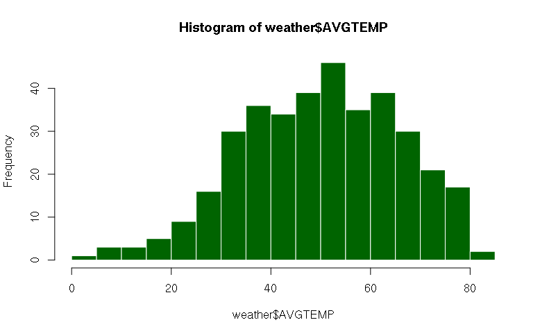
> hist(x = weather$AVGTEMP, col="darkgreen", border="white")
To see greater detail, you can increase the number of bars with the breaks parameter:
> hist(x = weather$AVGTEMP, breaks=20, col="darkgreen", border="white")
