Spatial Regression Analysis in R
Revised 15 June 2026
This tutorial demonstrates basic techniques for spatial regression analysis in R.
Example Data
The resource curse hypothesis asserts that countries with an abundance of oil, mineral or other natural resource wealth often have poorer economic and political environments than countries with fewer natural resources (Ross 1999).
The example in this tutorial uses spatial regression to investigate the validity of the resource curse.
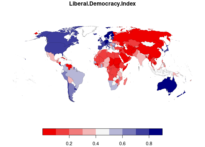
The independent variables are from a collection of indicators from the World Bank and the dependent variable is the V-Dem liberal democracy index which ranges from zero (autocracy) to one (liberal democracy).
library(sf)

countries = st_read("https://michaelminn.net/tutorials/data/2024-world-bank-indicators.geojson")

democracy = st_read("https://michaelminn.net/tutorials/data/2023-world-indices.geojson")

democracy = democracy[,c("ISO3", "Liberal.Democracy.Index", "Freedom.Score.2023")]

countries = merge(countries, st_drop_geometry(democracy), all.x=T, by.x = "Country_Code", by.y="ISO3")

countries = st_transform(countries, "ESRI:54030")

plot(countries["Liberal.Democracy.Index"], key.pos=1,
	border="#00000020",
	pal=colorRampPalette(c("red2", "whitesmoke", "navy")))
Ordinary Least Squares Linear Model
The first step is creating a non-spatial OLS linear model.
The independent variables assume that the dependency of the country on natural resources (Resource_Percent_GDP), the level of education (Percent_Secondary_School), and the level of overall development (GDP_per_Capita_PPP) should be predictive of the level of democracy.
model.ols = lm(Liberal.Democracy.Index ~ Resource_Percent_GDP
	+ Percent_Secondary_School + GDP_per_Capita_PPP, data=countries)

summary(model.ols)
While this is population rather than sampled data, the p-values hint that all of the variables except education make a meaningful contribution the model that predicts 40% of the variance in the democracy index.
Call:
lm(formula = Liberal.Democracy.Index ~ Resource_Percent_GDP +
    Percent_Secondary_School + GDP_per_Capita_PPP, data = countries)

Residuals:
     Min       1Q   Median       3Q      Max
-0.64722 -0.13930  0.01747  0.17584  0.40270

Coefficients:
                           Estimate Std. Error t value Pr(>|t|)
(Intercept)               2.758e-01  3.455e-02   7.982 1.36e-13 ***
Resource_Percent_GDP     -6.404e-03  1.493e-03  -4.289 2.86e-05 ***
Percent_Secondary_School  1.537e-03  7.218e-04   2.129   0.0345 *
GDP_per_Capita_PPP        3.915e-06  6.865e-07   5.702 4.49e-08 ***
---
Signif. codes:  0 ‘***’ 0.001 ‘**’ 0.01 ‘*’ 0.05 ‘.’ 0.1 ‘ ’ 1

Residual standard error: 0.2137 on 189 degrees of freedom
  (46 observations deleted due to missingness)
Multiple R-squared:  0.405,     Adjusted R-squared:  0.3956
F-statistic: 42.88 on 3 and 189 DF,  p-value: < 2.2e-16
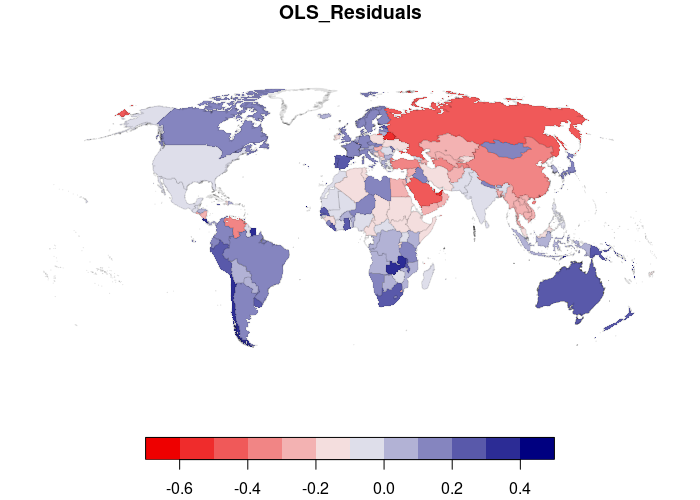
Mapping the residuals (actual - predicted) shows notable clusters of overpredicted levels in Asia and underpredicted levels in South America. This spatial autocorrelation violates the independence assumption of linear regression and will require spatial regression techniques to address.
countries$OLS_Residuals = NA

countries$OLS_Residuals[as.integer(names(ols$residuals))] = as.vector(model.ols$residuals)

plot(countries["OLS_Residuals"], key.pos=1,
	border="#00000020",
	pal=colorRampPalette(c("red2", "whitesmoke", "navy")))
Multicollinearity
Another assumption of ordinary least squares regression is that the independent variables are not correlated with each other.
Multicollinearity is when two or more independent variables in a regression model are correlated with each other in a way that biases the model coefficients and makes them unreliable.
We can use variance inflation factors (VIFs) to detect multicollinearity.
High VIFs (above five) indicate that a variable may have a problem with multicollinearity, which can be corrected by removing one of the correlated variables.
The vif() function from the Companion to Applied Regression (car) library lists VIF values for a model.
library(car)

print(vif(model.ols))
    Resource_Percent_GDP Percent_Secondary_School       GDP_per_Capita_PPP
                 1.00979                  1.88613                  1.89261
In this example, the VIFs are low, so multicollinearity is not a problem.
Transformation and Standardization
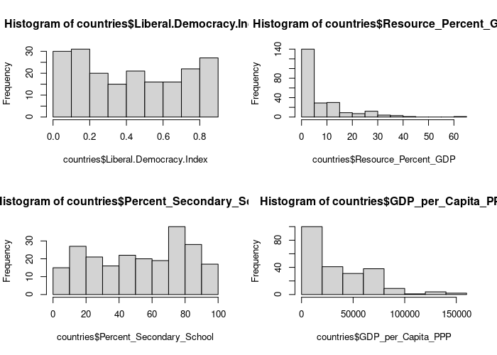
Another assumption of linear regresssion is that the variables are normally distributed. Histograms show resource dependence and GDP per capita are skewed.
par(mfrow=c(2,2))

hist(countries$Liberal.Democracy.Index)
hist(countries$Resource_Percent_GDP)
hist(countries$Percent_Secondary_School)
hist(countries$GDP_per_Capita_PPP)
In addition, variables need to be standardized to a common scale if you want to compare coefficients to each other evaluate the relative contribution of each variable to the model.
Transformation and standardization are combined into a function for convenience.
library(forecast)

transform_standardize = function(x) {
	x = x - min(x, na.rm=T) + 0.1

	x = BoxCox(x, lambda="auto")

	x = (x - mean(x, na.rm=T)) / sd(x, na.rm=T)
}

data = countries

data$Liberal.Democracy.Index = transform_standardize(data$Liberal.Democracy.Index)

data$Resource_Percent_GDP  = transform_standardize(data$Resource_Percent_GDP )

data$Percent_Secondary_School = transform_standardize(data$Percent_Secondary_School)

data$GDP_per_Capita_PPP = transform_standardize(data$GDP_per_Capita_PPP)
par(mfrow=c(2,2))

hist(data$Liberal.Democracy.Index)
hist(data$Resource_Percent_GDP)
hist(data$Percent_Secondary_School)
hist(data$GDP_per_Capita_PPP)
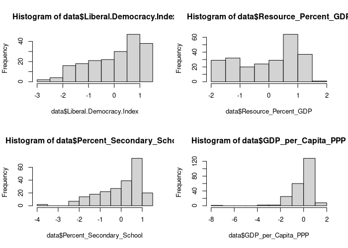
Standardization and transformation can change the variable relationships, and in this case also reduce the predictive strength of the lmodel (R-squared = .237 vs .396 untransformed).
model.std = lm(Liberal.Democracy.Index ~ Resource_Percent_GDP
	+ Percent_Secondary_School + GDP_per_Capita_PPP, data=data)

summary(model.std)
Call:
lm(formula = Liberal.Democracy.Index ~ Resource_Percent_GDP +
    Percent_Secondary_School + GDP_per_Capita_PPP, data = data)

Residuals:
    Min      1Q  Median      3Q     Max
-2.2680 -0.4567  0.2488  0.6286  1.3050

Coefficients:
                         Estimate Std. Error t value Pr(>|t|)
(Intercept)               0.12167    0.06298   1.932 0.054879 .
Resource_Percent_GDP     -0.24668    0.07395  -3.336 0.001024 **
Percent_Secondary_School  0.09003    0.08191   1.099 0.273135
GDP_per_Capita_PPP        0.29207    0.08417   3.470 0.000645 ***
---
Signif. codes:  0 ‘***’ 0.001 ‘**’ 0.01 ‘*’ 0.05 ‘.’ 0.1 ‘ ’ 1

Residual standard error: 0.8406 on 189 degrees of freedom
  (46 observations deleted due to missingness)
Multiple R-squared:  0.249,     Adjusted R-squared:  0.237
F-statistic: 20.88 on 3 and 189 DF,  p-value: 9.932e-12
Neighbors
In order to address autocorrelation between neighboring areas, we must first answer the ancient question, "Who is my neighbor?"
Neighboring areas can be defined by adjacency or proximity.
- Adjacency means that areas are considered neighbors if they share either a common border or a common corner (vertex). Adjacency based on a common vertex is called a queen rule after the rule in chess that allows queens to move diagonally. The poly2nb function can be used to find neighbors based on adjacency.
- Proximity means that areas are considered neighbors if they are within a specific distance of each other. The dnearneigh (within distance) and knearneigh (nearest k neighbors) can be used for proximity.
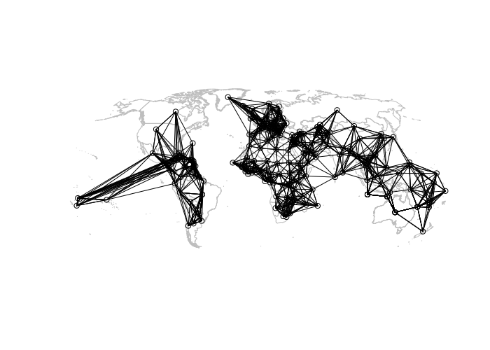
For this example we use knearneigh() function that defines a feature's neighbors as the closest k features.
library(spdep)

centroids = st_centroid(st_geometry(data))

nearest = knearneigh(as_Spatial(centroids), k=10)

neighbors = knn2nb(nearest)

weights = nb2listw(neighbors, style="W", zero.policy=T)

plot(st_geometry(data), border="gray")

plot(neighbors, coords=st_coordinates(st_centroid(data)), add=T)
Spatial Lag Regression
Spatial lag regression adds a model term that considers diffusion of the dependent variable across neighboring areas (Sparks 2015).
y = ρWY +βX + e
- y is the dependent variable.
- X is the matrix of independent variables.
- β is the vector of regression parameters to be estimated from the data.
- ρ is the autoregressive coefficient, which tells us how strong the resemblance is, on average, between Yi and it's neighbors.
- Y is the matrix of dependent variables.
- W is the spatial weight matrix that indicates indicates which the influence of neighbors.
- e is the error term.
The lagsarlm() function from the spatialreg library performs the regression. The first parameter is a formula specified in the same way as with lm(). The additional parameters (including the list of weights) are specific to spatial lag regression.
library(spatialreg)

model.lag = lagsarlm(Liberal.Democracy.Index ~ Resource_Percent_GDP +
    Percent_Secondary_School + GDP_per_Capita_PPP, data = data,
	listw=weights, tol.solve=1.0e-30, zero.policy=T)

summary(model.lag)
In this case, the high rho coefficient relative to the other coefficients indicates that the model is addressing autocorrelation in the dependent variable, but the relative relationship between the other coefficients is largely the same as the non-spatial OLS model.
The presence of a lag term means that the R-squared value from a lag model is inappropriate for determining fit. Spatial regression improves the reliability of coefficients rather than improving model fit.
Call:lagsarlm(formula = Liberal.Democracy.Index ~ Resource_Percent_GDP +
    Percent_Secondary_School + GDP_per_Capita_PPP, data = data,
    listw = weights, zero.policy = T, tol.solve = 1e-30)

Residuals:
     Min       1Q   Median       3Q      Max
-2.56988 -0.34631  0.13607  0.43283  1.31234

Type: lag
Coefficients: (asymptotic standard errors)
                          Estimate Std. Error z value Pr(>|z|)
(Intercept)               0.091485   0.052324  1.7484  0.08039
Resource_Percent_GDP     -0.148969   0.062200 -2.3950  0.01662
Percent_Secondary_School  0.048665   0.067980  0.7159  0.47407
GDP_per_Capita_PPP        0.175334   0.069237  2.5324  0.01133

Rho: 0.62453, LR test value: 66.349, p-value: 3.3307e-16
Asymptotic standard error: 0.066498
    z-value: 9.3917, p-value: < 2.22e-16
Wald statistic: 88.205, p-value: < 2.22e-16

Log likelihood: -205.1369 for lag model
ML residual variance (sigma squared): 0.46466, (sigma: 0.68166)
Number of observations: 193
Number of parameters estimated: 6
AIC: 422.27, (AIC for lm: 486.62)
LM test for residual autocorrelation
test value: 1.4461, p-value: 0.22916
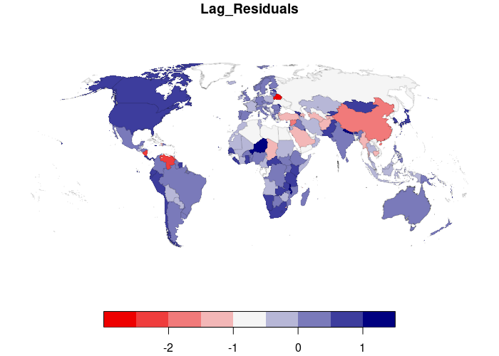
A map shows a reduction in residuals autocorrelation.
data$Lag_Residuals = NA

data$Lag_Residuals[as.integer(names(model.lag$residuals))] = as.vector(model.lag$residuals)

plot(data["Lag_Residuals"], key.pos=1,
	border="#00000020",
	pal=colorRampPalette(c("red2", "whitesmoke", "navy")))
Spatial Error Regression
In contrast to the focus of spatial lag regression on autocorrelation in the dependent variable, spatial error regression models spatial interactions in the independent variables (Eilers 2019).
y = βX + u
u = λWU + e
- y is the dependent variable.
- X is the matrix of independent variables.
- β is the vector of regression coefficients to be estimated from the data.
- u is the error term.
- λ is the autoregressive coefficient, which tells us how strong the autocorrelation of independent variables are with their neighbors.
- W is the spatial weights matrix that indicates indicates which areas are neighbors.
- U is the matrix of error terms.
- e is random error.
Spatial error regression is implemented in the errorsarlm(). function from the spatialreg library. This function uses the same parameters as the lagsarlm() function used for spatial lag regression above.
model.err = errorsarlm(Liberal.Democracy.Index ~ Resource_Percent_GDP +
    Percent_Secondary_School + GDP_per_Capita_PPP, data = data,
	listw=weights, tol.solve=1.0e-30, zero.policy=T)

summary(model.err)
With spatial error models, the error term is lambda (λ). As with rho above, the high lambda (0.37829) indicates that spatial autocorrelation is meaningful in this model.
Call:errorsarlm(formula = Liberal.Democracy.Index ~ Resource_Percent_GDP +
    Percent_Secondary_School + GDP_per_Capita_PPP, data = data,
    listw = weights, zero.policy = T, tol.solve = 1e-30)

Residuals:
     Min       1Q   Median       3Q      Max
-2.47646 -0.38082  0.12902  0.44856  1.24738

Type: error
Coefficients: (asymptotic standard errors)
                          Estimate Std. Error z value Pr(>|z|)
(Intercept)               0.180730   0.155338  1.1635 0.244642
Resource_Percent_GDP     -0.248489   0.076387 -3.2530 0.001142
Percent_Secondary_School  0.152887   0.076281  2.0043 0.045042
GDP_per_Capita_PPP        0.211160   0.073859  2.8590 0.004250

Lambda: 0.69056, LR test value: 73.376, p-value: < 2.22e-16
Asymptotic standard error: 0.06577
    z-value: 10.5, p-value: < 2.22e-16
Wald statistic: 110.24, p-value: < 2.22e-16

Log likelihood: -201.6235 for error model
ML residual variance (sigma squared): 0.44049, (sigma: 0.66369)
Number of observations: 193
Number of parameters estimated: 6
AIC: NA (not available for weighted model), (AIC for lm: 486.62)
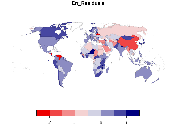
A map shows some reduction in residuals autocorrelation.
data$Err_Residuals = NA

data$Err_Residuals[as.integer(names(model.err$residuals))] = as.vector(model.err$residuals)

plot(data["Err_Residuals"], key.pos=1,
	border="#00000020",
	pal=colorRampPalette(c("red2", "whitesmoke", "navy")))
Choosing Between Spatial Lag and Spatial Error
You can choose between models based on your understanding of the phenomenon being modeled, although such a choice assumes a level of accurate understanding that will likely not be present if you are performing this kind of modeling.
A more quantifiably justifiable selection method is to choose the model with the best fit. The Akaike information criterion (AIC) is an estimate of model prediction error, with lower values representing lower information loss (Akaike 1974; Wikipedia 2022). In choosing between models, the model with the lower AIC is the model with the better fit.
The AIC() function from the built-in stats library displays the AIC values for the three models. The lowest value is the OLS model, so it would be the most appropriate model to use.
AIC(model.ols)
[1] -41.97011

AIC(model.lag)
[1] 422.2739

AIC(model.error)
[1] 415.247
Another option for comparing spatial models is to use the Lagrange multiplier test (LMT) (i.e. score test). The LMT is implemented in the spatialreg library with the lm.LMtests() function. The model with the lowest Lagrange multiplier value is the best-fitting model.
In the listing below, the LMT is inconsistent with the AIC comparisons above, since the LM for the error model (LMerr = 127.47) is higher than the lag model (LMlag = 114.28).
The all listing also includes entries for versions of the lag (RLMlag) and error (RLMerr) models that are "robust" to the presence of both lag and error.
lm.LMtests(model.ols, listw=weights, test="all")
        Lagrange multiplier diagnostics for spatial dependence

data:
model: lm(formula = Liberal.Democracy.Index ~ Resource_Percent_GDP +
Percent_Secondary_School + GDP_per_Capita_PPP, data = countries)
weights: weights

LMerr = 127.47, df = 1, p-value < 2.2e-16


        Lagrange multiplier diagnostics for spatial dependence

data:
model: lm(formula = Liberal.Democracy.Index ~ Resource_Percent_GDP +
Percent_Secondary_School + GDP_per_Capita_PPP, data = countries)
weights: weights

LMlag = 114.28, df = 1, p-value < 2.2e-16
Global Moran's I
You can verify autocorrelation has been removed from the residuals using the Global Moran's I statistic, developed by Patrick Alfred Pierce Moran (1950).
Global Moran's I assesses autocorrelation over the entire area of analysis as a single number. Values of the global Moran's I statistic vary from -1 (evenly dispersed = evenly spread out) to 0 (no autocorrelation) to +1 (completely clustered).
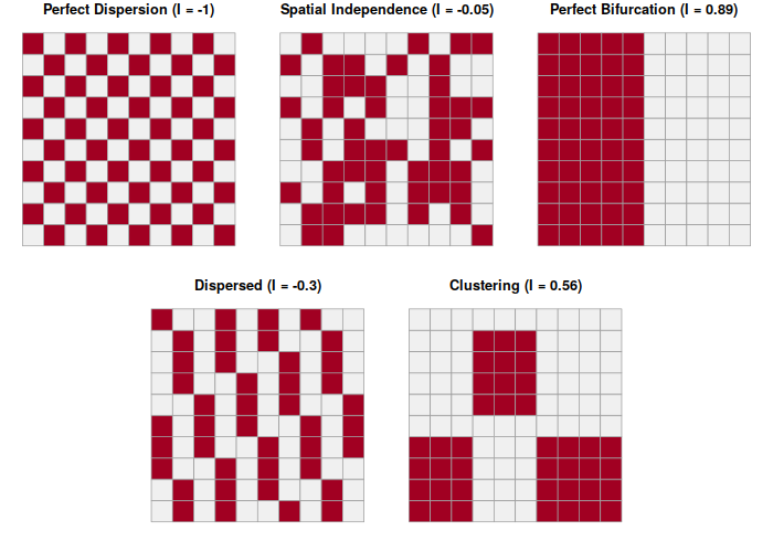
Once you have a weights list (see above), moran.test() calculates the Moran's I statistic for the residuals being analyzed.
As expected, the OLS residuals have higher I values than the spatial model residuals.
moran.ols = moran.test(data$OLS_Residuals, weights, na.action=na.omit)

print(moran.ols)
Moran I statistic standard deviate = 11.748, p-value < 2.2e-16
alternative hypothesis: greater
sample estimates:
Moran I statistic       Expectation          Variance
      0.379265864      -0.005208333       0.001071074
moran.lag = moran.test(data$Lag_Residuals, weights, na.action=na.omit)

print(moran.lag)
Moran I statistic standard deviate = 0.86573, p-value = 0.1933
alternative hypothesis: greater
sample estimates:
Moran I statistic       Expectation          Variance
      0.023038741      -0.005208333       0.001064596
moran.err = moran.test(data$Err_Residuals, weights, na.action=na.omit)

print(moran.err)
Moran I statistic standard deviate = -0.66342, p-value = 0.7465
alternative hypothesis: greater
sample estimates:
Moran I statistic       Expectation          Variance
     -0.026856967      -0.005208333       0.001064828