Simulated Data With R
R has a wide variety of capabilities for generating simulated data that can be useful for testing or pedagogy.
Linear Sequences
Linear sequences of numbers are commonly used in R, notably for iterating through members of data structures.
For sequences of successive integers, the colon operator is usually the simplest choice. The result is all integers between the number before the colon and the number after the colon, inclusive. The sequence can be ascending or descending:
> x = 1:10
> x
 [1]  1  2  3  4  5  6  7  8  9 10
> x = 1:-10
> x
 [1]   1   0  -1  -2  -3  -4  -5  -6  -7  -8  -9 -10
> x = -1:10
> x
 [1] -1  0  1  2  3  4  5  6  7  8  9 10
> x = 1:1
> x
[1] 1
For sequences of real numbers or sequences that proceed in increments not equal to one, the seq(from, to, by) function:
> x = seq(10, 12, 0.3)
> x
[1] 10.0 10.3 10.6 10.9 11.2 11.5 11.8

> x = seq(-10, -12, -0.3)
> x
[1] -10.0 -10.3 -10.6 -10.9 -11.2 -11.5 -11.8
For regular sequences of specific numbers the rep() (repeat) function can be used. The parameters are:
- x: the value to repeat
- times: the number of times to repeat that value
> x = rep(1, 10)
> x
 [1] 1 1 1 1 1 1 1 1 1 1
Multiple calls can be concatenated with the c() function to create collections of numbers or categorical/dichotomous data:
> x = c(rep(1,10), rep(2, 10), rep(3, 10))
> x
 [1] 1 1 1 1 1 1 1 1 1 1 2 2 2 2 2 2 2 2 2 2 3 3 3 3 3 3 3 3 3 3
> x = c(rep("Democratic", 4), rep("Republican", 6))
> x
 [1] "Democratic" "Democratic" "Democratic" "Democratic" "Republican"
 [6] "Republican" "Republican" "Republican" "Republican" "Republican"
Nonlinear Sequences
Linear sequences can be transformed to nonlinear sequences of numbers using a variety of functions. Some examples are given below.
Exponential and Logarithmic Sequences
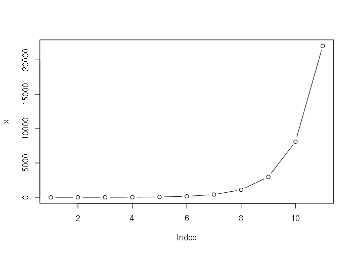
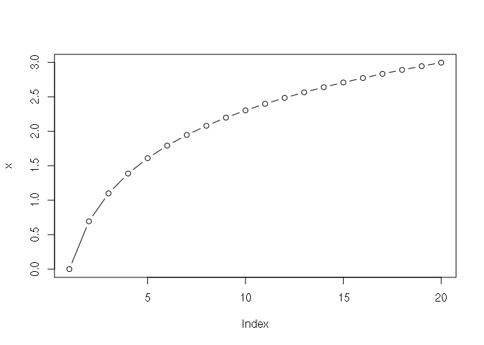
Many phenomena, such as growth, follow exponential or logarithmic curves. Natural exponentials and logarithms (powers and roots of Euler's Number) are supported with the exp() and log() functions.
> x = exp(0:10)
> x
 [1]     1.000000     2.718282     7.389056    20.085537    54.598150
 [6]   148.413159   403.428793  1096.633158  2980.957987  8103.083928
[11] 22026.465795
> plot(x, type="b")
> x = log(1:20)
> x
 [1] 0.0000000 0.6931472 1.0986123 1.3862944 1.6094379 1.7917595 1.9459101
 [8] 2.0794415 2.1972246 2.3025851 2.3978953 2.4849066 2.5649494 2.6390573
[15] 2.7080502 2.7725887 2.8332133 2.8903718 2.9444390 2.9957323
> plot(x, type="b")
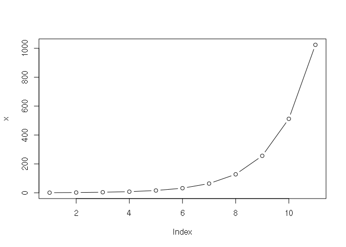
Exponential sequences can be created based on any base using the carat operator:
> x = 2^(0:10)
> x
 [1]    1    2    4    8   16   32   64  128  256  512 1024
> plot(x, type="b")
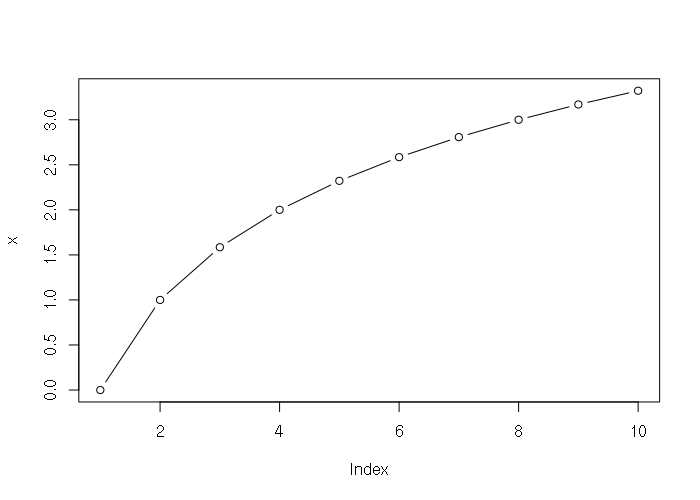
The optional second parameter to the log() function is an base if you need a logarithm on something other than e:
> x = log(1:10, 2)
> x
 [1] 0.000000 1.000000 1.584963 2.000000 2.321928 2.584963 2.807355 3.000000
 [9] 3.169925 3.321928
> plot(x, type="b")
Cyclical Sequences
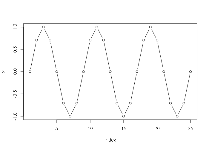
Many phenomena such as temperature or market activity occur in regularly repeating cycles. The sin() and cos() functions can be used to create cyclical sequences. The parameter is in radians (multiples of 2π), and the native pi constant can be used to convert a linear sequence to radians:
> x = sin(seq(0, 6, 0.25) * pi)
> x
 [1]  0.000000e+00  7.071068e-01  1.000000e+00  7.071068e-01  1.224647e-16
 [6] -7.071068e-01 -1.000000e+00 -7.071068e-01 -2.449294e-16  7.071068e-01
[11]  1.000000e+00  7.071068e-01  3.673940e-16 -7.071068e-01 -1.000000e+00
[16] -7.071068e-01 -4.898587e-16  7.071068e-01  1.000000e+00  7.071068e-01
[21]  6.123234e-16 -7.071068e-01 -1.000000e+00 -7.071068e-01 -7.347881e-16
> plot(x, type="b")
Normally-Distributed Sequences
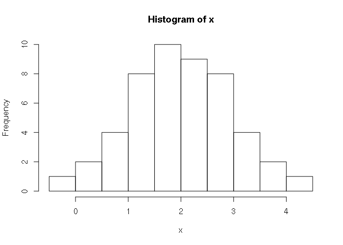
A normally distributed sequence of numbers can be created using the qnorm() quantile function. The parameters:
- x: A linear sequence of probabilities in the range 0 to 1
- mean: The mean (μ)
- sd: The standard deviation (σ)
> x = qnorm(seq(0, 1, 0.02), 2, 1)
> x
 [1]        -Inf -0.05374891  0.24931393  0.44522641  0.59492844  0.71844843
 [7]  0.82501321  0.91968066  1.00554212  1.08463491  1.15837877  1.22780679
[13]  1.29369744  1.35665459  1.41715849  1.47559949  1.53230120  1.58753687
[19]  1.64154121  1.69451921  1.74665290  1.79810652  1.84903078  1.89956628
[25]  1.94984642  2.00000000  2.05015358  2.10043372  2.15096922  2.20189348
[31]  2.25334710  2.30548079  2.35845879  2.41246313  2.46769880  2.52440051
[37]  2.58284151  2.64334541  2.70630256  2.77219321  2.84162123  2.91536509
[43]  2.99445788  3.08031934  3.17498679  3.28155157  3.40507156  3.55477359
[49]  3.75068607  4.05374891         Inf
> hist(x)
Sequences Based on Percentiles
You will occasionally find statistical data given as percentiles. For example, in this document the CDC gives the following percentiles for the height of men in the USA:
Percentile:	5     10    15    25    50    75    85    90    95
Height (in):    64.3  65.4  66.1  67.2  69.1  71.2  72.3  73.0  74.1
This means that 5% of men are below 64.3 inches, 25% are below 67.2 inches, etc.
By using a spline, it is possible to simulate a curve that fits those percentile points, then use the predict() function to create a representative sample. The CDC indicates that they based their estimates on 5,232 examined persons (sample size), which is what is simulated below:
# Table 12.  Height in inches for males aged 20 and over and number of examined
# persons, mean, standard error of the mean, and selected percentiles, by race
# and Hispanic origin and age: United States, 2011–2014

pheight = c(64.3, 65.4, 66.1, 67.2, 69.1, 71.2, 72.3, 73.0, 74.1)
percentile = c(5, 10, 15, 25, 50, 75, 85, 90, 95)

# Create a spline to fit those points
spline = smooth.spline(percentile, pheight)

# Simulate 5,232 points that cover the range of percentiles
height = predict(spline, 100 * (1:5232) / 5233)

# Plot the simulated data
plot(percentile, pheight, col="blue", pch=16)
lines(height$x, height$y)

# Print the descriptive statistics
paste("mean = ", mean(height$y))
paste("stdev =", sd(height$y))
paste("stderr =", sd(height$y) / sqrt(length(height$y)))
Logistic Sequences
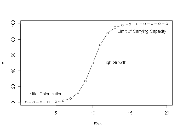
Phenomena like growth to the carrying capacity of an ecosystem follow a logistic curve, which can be generated using the self-starting logistic model function SSlogis(). The parameters are:
- input: A linear sequence
- Asym: The maximum output value (carrying capacity)
- xmid: The x value that is at the middle of the curve
- scal: The scaling (width) of the curve
> x = SSlogis(1:20, Asym = 100, xmid = 10, scal = 1)
> x
 [1]  0.01233946  0.03353501  0.09110512  0.24726232  0.66928509  1.79862100
 [7]  4.74258732 11.92029220 26.89414214 50.00000000 73.10585786 88.07970780
[13] 95.25741268 98.20137900 99.33071491 99.75273768 99.90889488 99.96646499
[19] 99.98766054 99.99546021
> plot(x, type="b")
> text(1, 10, "Initial Colonization", pos=4)
> text(11, 50, "High Growth", pos=4)
> text(13, 90, "Limit of Carrying Capacity", pos=4)
Random Sequences
Random sequences of numbers are useful for testing analysis code, and are essential for formal statistical techniques like Monte Carlo methods.
Random sequences of numbers do not follow a regular pattern. While computers are deterministic machines that cannot generate truly random sequences of numbers, there are a variety of algorithms that generate pseudo-random sequences that are close enough to random to meet the needs of researchers.
Uniformly-Distributed Random Sequences
The most basic random number generating function is the runif() function, which generates a random sequence in a uniform distribution (the unif part of the name). The parameters:
- n: The count of numbers to generate
- min: The minimum possible value in the sequence (defaults to 0)
- max: The maximum possible value in the sequence (defaults to 1)
> x = runif(20)
> x
 [1] 0.6877721 0.7481171 0.9397808 0.6928701 0.6112946 0.4786213 0.3839646
 [8] 0.4164434 0.9205573 0.8799462 0.1750195 0.5641760 0.9437534 0.5265315
[15] 0.1380678 0.8415553 0.4562519 0.8806186 0.9218461 0.3643150
> hist(x)
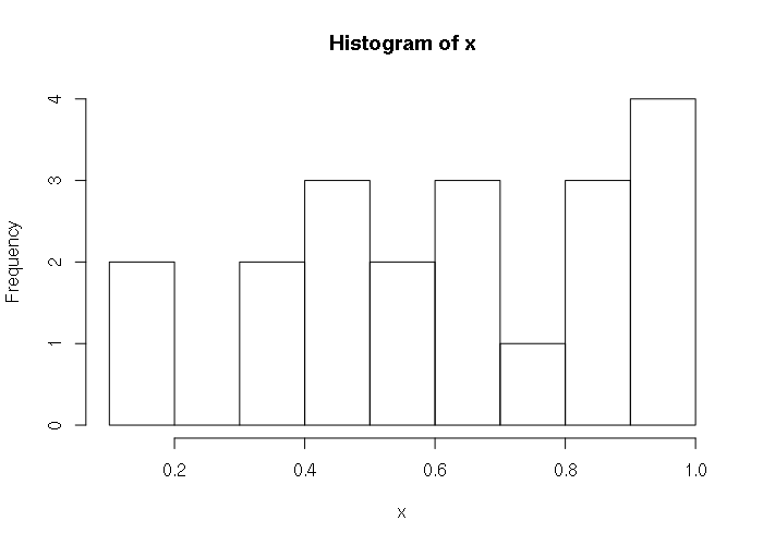
runif() will return an unpredictably different sequence on each successive call. If you need consistent repeatability, such as for a demonstration presentation, you can use the set.seed() function to set a seed number that is used to start the random number generator at a specific point:
> set.seed(1)
> runif(10)
 [1] 0.26550866 0.37212390 0.57285336 0.90820779 0.20168193 0.89838968
 [7] 0.94467527 0.66079779 0.62911404 0.06178627
> runif(10)
 [1] 0.2059746 0.1765568 0.6870228 0.3841037 0.7698414 0.4976992 0.7176185
 [8] 0.9919061 0.3800352 0.7774452
> set.seed(1)
> runif(10)
 [1] 0.26550866 0.37212390 0.57285336 0.90820779 0.20168193 0.89838968
 [7] 0.94467527 0.66079779 0.62911404 0.06178627
Normally-Distributed Random Sequences
As with linear sequences, a random sequence generated by runif() can be fed into other functions to transform to a different distribution. There are also convenience functions that do this in one step. For example the rnorm() function generates random numbers that have a normal distribution. Because the sequence is random, the distribution will not be perfectly even.
For example, the mean height of men in the US is 5 feet, 9.3 inches with a standard deviation of 2.94 inches.. Simulated height for 50 men:
> x = rnorm(50, (5 * 12) + 93, 2.94)
> x
 [1] 153.4227 152.6538 150.3185 148.7735 150.6566 156.6870 155.2701 152.3546
 [9] 151.7511 151.7682 155.9311 152.1892 156.6927 154.9012 156.8200 150.4326
[17] 153.0246 150.4102 154.7530 153.3520 152.1704 157.2806 153.6733 155.9298
[25] 155.2987 150.7163 151.1890 153.1369 149.6767 154.6956 149.2346 157.7788
[33] 151.5280 157.9342 151.7872 150.1415 153.0746 153.0808 148.0603 156.0980
[41] 149.7084 153.9867 154.4547 153.4059 152.6508 153.5812 149.8580 150.6386
[49] 149.7255 157.6455
> hist(x, breaks=10)
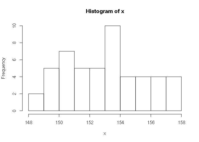
Random Integers
runif() generates real numbers. If you need a random sequence of integers (whole numbers), the round() function can be used with the as.integer() type convertor. Because the sequence is random, it will not necessarily be completely even:
> x = as.integer(round(runif(50, 0, 10)))
> x
 [1]  2  7  6  2  0  7  1  5  7  4  8  1  9 10  1  1  0 10  8  9  2  6  8  5 10
[26] 10  3 10  8  5  6  4  4 10 10  5  2  2  1  1  5  6  1  2  1  8  9  1  8  3
> hist(x, breaks=11)
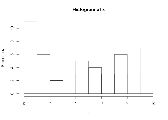
Random Categorical Data
Random dichotomous (one of two values) sequences can be created using the ifelse() function. The condition determines the proportion of values, although with small numbers the randomness of the sequence may not match the proportion:
> x = ifelse(runif(20) > 0.6, "Democratic", "Republican")
> x
 [1] "Republican" "Democratic" "Republican" "Republican" "Republican"
 [6] "Republican" "Republican" "Republican" "Democratic" "Republican"
[11] "Democratic" "Republican" "Republican" "Republican" "Democratic"
[16] "Republican" "Republican" "Democratic" "Republican" "Democratic"
> table(x)
x
Democratic Republican
         6         14
Random Sampling
Random numbers are commonly used to select a random sample from a list of possible people to survey. The sample() function is a shortcut to perform this task. As with runif(), the set.seed() function can be used to get reproducable results. The parameters to sample():
- x: a vector of values to sample from
- size: the number of values to sample
> people = c("Hailey", "Tom", "Jane", "Jim", "Tony", "Mike",
+         "Ethan", "Misty", "Frank", "Joan", "Ida", "Helen")
> set.seed(1)
> sample(people, 5)
[1] "Jim"   "Tony"  "Mike"  "Frank" "Tom"
> sample(people, 5)
[1] "Ida"    "Helen"  "Ethan"  "Mike"   "Hailey"
> set.seed(1)
> sample(people, 5)
[1] "Jim"   "Tony"  "Mike"  "Frank" "Tom"
sample() can be used to demonstrate the margin of error with sampling. For example, in close election involving 10,000 voters, with 51 percent voting for a Democratic candidate, three successive random samples give significantly different results, including results outside the ±5% margin of error with a 95% level of confidence:
# Simulated population of 10,000 voters with 51% planning to vote Democratic
> x = c(rep("Republican", 4900), rep("Democratic", 5100))
> set.seed(1)
> table(sample(x, 100))

Democratic Republican
        50         50
> table(sample(x, 100))

Democratic Republican
        55         45
> table(sample(x, 100))

Democratic Republican
        41         59
While political polling is an art that is more complex than simple random sampling, this helps demonstrate how polls that incorporate rigorous sampling methodologies can yield predictions that do not match the final election results.
Two-Variable Relationship Example
The following formula is use in linear regression to model the relationship between two variables:
Yi = α + ΒXi + εi
In English that can be described as:
y = offset + scale * sequence + random_error
For example, there is a rough inverse correlation (R2) between median household income and percent obesity in US counties (2017-county-data.csv):
> x = read.csv("2017-county-data.csv")
> plot(x$MEDHHINC, x$PCOBESITY, col="#00000080")
> m = lm(PCOBESITY ~ MEDHHINC, data=x)
> abline(m)
> abline(m, col="darkred")
> summary(m)

Call:
lm(formula = PCOBESITY ~ MEDHHINC, data = x)

Residuals:
     Min       1Q   Median       3Q      Max
-15.8543  -2.1624   0.2542   2.5016  11.8794

Coefficients:
              Estimate Std. Error t value Pr(>|t|)
(Intercept)  3.922e+01  2.752e-01  142.51   <2e-16 ***
MEDHHINC    -1.767e-04  5.684e-06  -31.09   <2e-16 ***
---
Signif. codes:  0 ‘***’ 0.001 ‘**’ 0.01 ‘*’ 0.05 ‘.’ 0.1 ‘ ’ 1

Residual standard error: 3.9 on 3137 degrees of freedom
  (8 observations deleted due to missingness)
Multiple R-squared:  0.2355,    Adjusted R-squared:  0.2353
F-statistic: 966.5 on 1 and 3137 DF,  p-value: < 2.2e-16
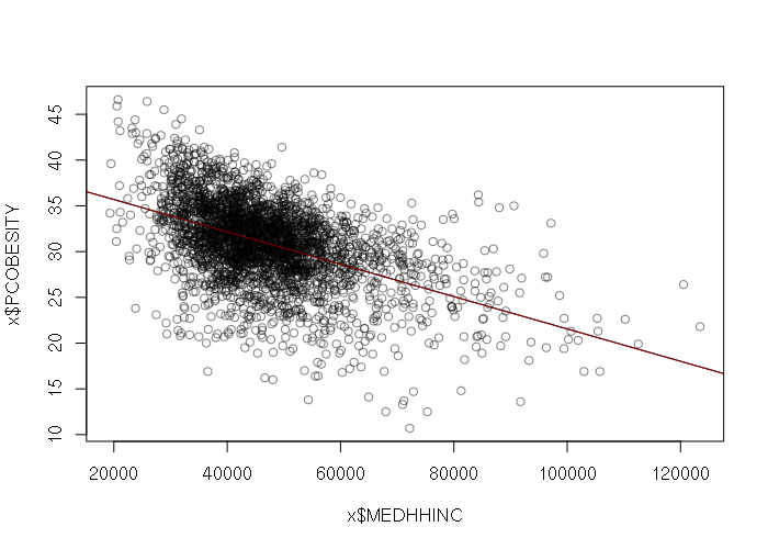
That relationship can be described by the following formula. For each dollar increase in median household income, the percent of obese residents drops by 0.018 percent.
percent_obesity = 39.22 - 0.0001767 * median_household_income
Given that formula we can combine functions described above to create simulated data. Also included is a simple linear model (lm()) to verify the results.
> income = seq(0, 150000, 150)
> error = runif(length(income), -5, 5)
> set.seed(1)
> pcobesity = 39.22 - (0.0001767 * income) + error
> plot(income, pcobesity)
>
> # Verify the simulated data with a linear model
> model = lm(pcobesity ~ income)
> summary(model)

Call:
lm(formula = pcobesity ~ income)

Residuals:
    Min      1Q  Median      3Q     Max
-5.0612 -2.2972 -0.1046  2.2012  4.8564

Coefficients:
              Estimate Std. Error t value Pr(>|t|)
(Intercept)  3.945e+01  4.377e-01   90.13   <2e-16 ***
income      -1.781e-04  5.046e-06  -35.30   <2e-16 ***
---
Signif. codes:  0 ‘***’ 0.001 ‘**’ 0.01 ‘*’ 0.05 ‘.’ 0.1 ‘ ’ 1

Residual standard error: 2.703 on 149 degrees of freedom
Multiple R-squared:  0.8932,    Adjusted R-squared:  0.8925
F-statistic:  1246 on 1 and 149 DF,  p-value: < 2.2e-16
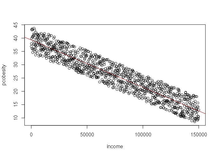
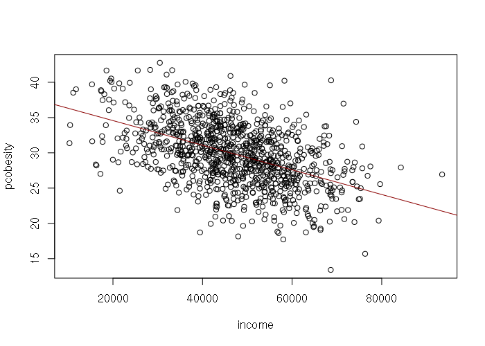
However, income by county is normally rather than uniformly distributed, suggesting that rnorm() would be better than runif() for generating the input values and error values for the model:
> set.seed(1)
> income = rnorm(1000, mean=47000, sd=12200)
> error = rnorm(length(income), -1, 3.9)
> pcobesity = 39.22 - (0.0001767 * income) + error
> plot(income, pcobesity)
>
> # Verify the simulated data with a linear model
> model = lm(pcobesity ~ income)
> abline(model, col="darkred")
> summary(model)

Call:
lm(formula = pcobesity ~ income)

Residuals:
     Min       1Q   Median       3Q      Max
-12.6689  -2.6206  -0.0536   2.9460  14.2129

Coefficients:
              Estimate Std. Error t value Pr(>|t|)
(Intercept)  3.806e+01  4.934e-01   77.13   <2e-16 ***
income      -1.746e-04  1.017e-05  -17.18   <2e-16 ***
---
Signif. codes:  0 ‘***’ 0.001 ‘**’ 0.01 ‘*’ 0.05 ‘.’ 0.1 ‘ ’ 1

Residual standard error: 4.058 on 998 degrees of freedom
Multiple R-squared:  0.2281,    Adjusted R-squared:  0.2274
F-statistic:   295 on 1 and 998 DF,  p-value: < 2.2e-16
