Representing Data in R
Data Types
Computers represent everything internally as numbers, but R, like most programming languages, provides a variety of fundamental data types to make the representation of data that a user sees closer to the way that data is used to represent reality.
Integers
Integers are whole numbers no decimal points. They are commonly used for counts (such as population) and for indexing elements in data structures (explained below).
> x = 1 + 1
> x
[1] 2
Real Numbers (Floating Point)
Real numbers are numbers that can have decimal points. R uses the type named double for real numbers. Real numbers are used for everything that can be represented quantitatively.
> x = 1.1 + 1.0
> x
[1] 2.1
> typeof(x)
[1] "double"
Character Strings
Character data is text data with letters and words. Character data in other languages are often called strings for strings of characters. Character data needs to be enclosed in double or single quotes to make it clear to the software where the text begins and ends.
> x = "Hello, world!"
> x
[1] "Hello, world!"
> typeof(x)
[1] "character"
Logical Values
Logical values can be either TRUE or FALSE. TRUE and FALSE can be abbreviated with the letters T or F.
Logical values are commonly created as the result of comparisons, and used to select items from structures or make decisions about program flow.
> 5 > 7
[1] FALSE
> 5 < 7
[1] TRUE
Factors
Factor data is a numeric representation of text data. Factors are commonly used internally by R for categorical data to make such data easier to process and compare.
> x = as.factor(c("Alpha", "Beta", "Gamma", "Delta", "Alpha"))
> x
[1] Alpha Beta  Gamma Delta Alpha
Levels: Alpha Beta Delta Gamma
> as.integer(x)
[1] 1 2 4 3 1
> typeof(x)
[1] "integer"
Dates
Dates are also represented internally by R as numbers. While dates can be represented as character data, if you want to be able to sort or order by date, use of the date data type is helpful. Date and time handling in R is a bit messy (because the way humans write dates and times are inconsistent), and you should consult this description from Berkeley for more information.
> x = as.Date("2017-01-01")
> x
[1] "2017-01-01"
> as.integer(x)
[1] 17167
> typeof(x)
[1] "double"
> class(x)
[1] "Date"
Data Structures
R is a program for statistical analysis, and most statistical data exists in collections like tables or matrices. R uses a variety of data structures to keep collections of data together in a useful manner.
| Name | Dimensions | Data Types |
|---|---|---|
| Vector | 1 | 1 |
| Matrix | 2 | 1 |
| Array | 1+ | 1 |
| List | 1 | Mixed |
| Data Frame | 1+ | 1+ |
| Time Series | 2 | 2+ |
Vectors
Vectors are one-dimensional collections of data of the same data type. Values that are not in other types of data structures are probably vectors. Variables with one value are vectors of length one.

Creation
Vectors can be created by enclosing individual values separated by commas as parameters to the c() combine function:
> x = c(1, 3, 5, 6, 7)
> x
[1] 1 3 5 6 7
> y = c('Joe', 'Frank', 'Tom')
> y
[1] "Joe"   "Frank" "Tom"
Visualization
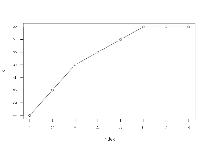
Numeric vectors can be visualized as line graphs with the plot() function:
> x = c(1, 3, 5, 6, 7, 8, 8, 8)
> plot(x, type='b')
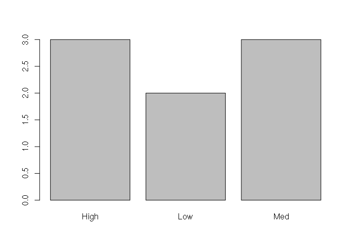
Character vectors of categorical data can be summarized into tables with the table() function, and those tables can be visualized using the barplot() function.
> states = c("LA", "MS", "AL", "NY", "OH", "VA", "CA", "CO")
> obesity = c("High", "High", "High", "Med", "Med", "Med", "Low", "Low")
> names(obesity) = states
> obesity
    LA     MS     AL     NY     OH     VA     CA     CO
"High" "High" "High"  "Med"  "Med"  "Med"  "Low"  "Low"
> table(obesity)
obesity
High  Low  Med
   3    2    3
> barplot(table(obesity))
Access and Subsetting
The length of a vector is returned by the length() function.
Individual elements or groups of elements can be accessed with numeric indexes inside square brackets, with index 1 being the first element in the vector. Indexes can also be sequences or vectors.
> x = c('Vanilla', 'Chocolate', 'Strawberry', 'Avocado', 'Anchovy')
> length(x)
[1] 5
> x[1]
[1] "Vanilla"
> x[3:5]
[1] "Strawberry" "Avocado"    "Anchovy"
> x[3:length(x)]
[1] "Strawberry" "Avocado"    "Anchovy"
> x[c(1,3,4)]
[1] "Vanilla"    "Strawberry" "Avocado"
The elements of a vector can be named using the names() function, and the elements accessed with either those names or numeric indices.
> x = c('Vanilla', 'Chocolate', 'Strawberry', 'Avocado', 'Anchovy')
> x[1]
[1] "Vanilla"
> x[3:5]
[1] "Strawberry" "Avocado"    "Anchovy"
> x[c(1,3,4)]
[1] "Vanilla"    "Strawberry" "Avocado"
> names(x) = c('Alpha', 'Beta', 'Gamma', 'Delta', 'Epsilon')
> x
       Alpha         Beta        Gamma        Delta      Epsilon
   "Vanilla"  "Chocolate" "Strawberry"    "Avocado"    "Anchovy"
> x['Beta']
       Beta
"Chocolate"
> x[2]
       Beta
"Chocolate"
Appending and Deleting
Elements can be appended to the beginning or ending of a vector by including the vector within another c() function. Elements can be deleted by setting the vector to a subset.
> x = c('Joe', 'Frank', 'Tom')
> x
[1] "Joe"   "Frank" "Tom"
> x = c('Mary', x)
> x
[1] "Mary"  "Joe"   "Frank" "Tom"
> x = c(x, 'Hailey')
> x
[1] "Mary"   "Joe"    "Frank"  "Tom"    "Hailey"
> x = x[1:3]
> x
[1] "Mary"  "Joe"   "Frank"
Operations
One of the strengths of R is the ability to perform operations all elements of a vector (or other data structure) with single statements:
> x = c(1, 3, 5, 6, 7)
> y = c(100, 200, 300, 400, 500)
> x + y
[1] 101 203 305 406 507
> x * y
[1]  100  600 1500 2400 3500
> x + 1
[1] 2 4 6 7 8
> sum(x)
[1] 22
Data Frames
A data frame is a two-dimensional data structure arranged into rows and columns like a spreadsheet. The structure can contain multiple data types, but all elements in a single column must be the same data type.
Creation
Data frames can be created directly from vectors using the data.frame() function.
> names = c('LA', 'MS', 'AL', 'NY', 'OH', 'VA', 'CA', 'CO')
> obesity = c('High', 'High', 'High', 'Med', 'Med', 'Med', 'Low', 'Low')
> density = c(106, 64, 95, 416, 283, 207, 244, 50)
> states = data.frame(names, obesity, density)
> states
  names obesity density
1    LA    High     106
2    MS    High      64
3    AL    High      95
4    NY     Med     416
5    OH     Med     283
6    VA     Med     207
7    CA     Low     244
8    CO     Low      50
Import and Export
Data frames are commonly imported from comma-separated-value (CSV) files using the read.csv() function. CSV files can be created in and exported from spreadsheet programs like Excel. The as.is=T parameter prevents the function from converting character strings to factors, which makes them easier to display. The CSV file for this example can be downloaded HERE.
> states = read.csv('2017-state-data.csv', as.is=T)
> states
   ST                State WIN2012 DEM2012 PCDEM2012 GOP2012 PCGOP2012 WIN2016
1  AK               Alaska  Romney   91696      41.6  121234      55.0   Trump
2  AL              Alabama  Romney  793620      38.4 1252453      60.7   Trump
3  AR             Arkansas  Romney  391953      36.9  643717      60.6   Trump
4  AZ              Arizona  Romney  900081      44.1 1107130      54.2   Trump
5  CA           California   Obama 6241648      59.2 4046524      38.4 Clinton
6  CO             Colorado   Obama 1238490      51.2 1125391      46.5 Clinton
7  CT          Connecticut   Obama  912531      58.4  631432      40.4 Clinton
8  DC District of Columbia   Obama  222332      91.4   17337       7.1 Clinton
9  DE             Delaware   Obama  242547      58.6  165476      40.0 Clinton
...
Data frames can be written to CSV files using the analogous write.csv() function.
Visualization
The parallel cross-sectional or time-series data in a data frame permits a wide variety of different visualizations of relationships between columns, only a handful of which are covered here.
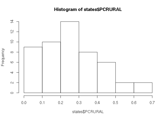
Single columns can be visualized using the same visualizations used with vectors.
> states = read.csv('2017-state-data.csv')
> hist(states$PCRURAL)
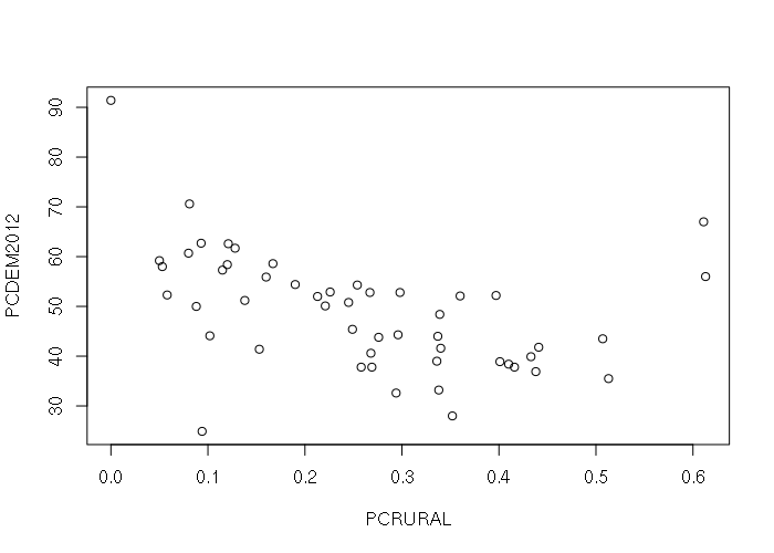
The default plot() of a data frame with two numeric columns creates an X-Y scatter plot, with the leftmost column as the X-axis:
plot(states[,c('PCRURAL', 'PCDEM2012')])
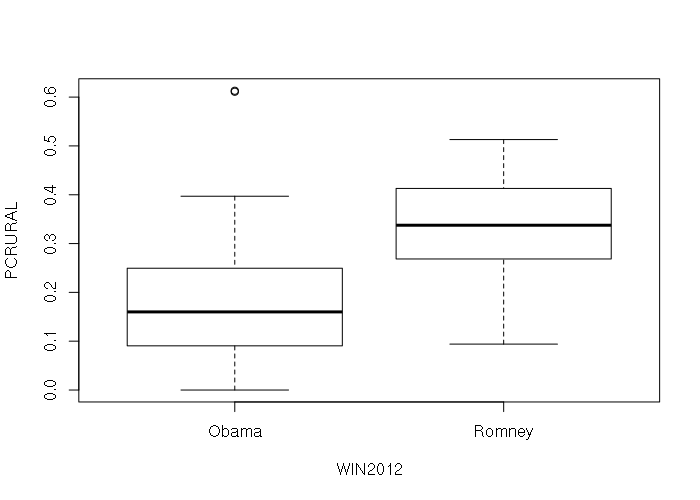
The default plot() of a data frame with a categorical and numeric column creates a boxplot giving the ranges of values in each category:
plot(states[,c('WIN2012', 'PCRURAL')])
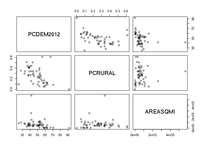
The default plot() of a data frame with multiple numeric columns is a pairplot with X-Y scatter plots for all possible pairs of columns that can be used to investigate possible relationships between variables.
plot(states[,c('PCDEM2012', 'PCRURAL', 'AREASQMI')])
Access and Subsetting
As with vectors, elements can be accessed with numeric indices inside square brackets, with the first number as the row number and the second number as the column number, starting with 1 as the top row or leftmost column. Numbers can be ranges of numbers or vectors of numbers. An entire row or all columns can be accessed by leaving the numeric index blank.
> names = c('LA', 'MS', 'AL', 'NY', 'OH', 'VA', 'CA', 'CO')
> obesity = c('High', 'High', 'High', 'Med', 'Med', 'Med', 'Low', 'Low')
> density = c(106, 64, 95, 416, 283, 207, 244, 50)
> states = data.frame(names, obesity, density)

> dim(states)
[1] 8 3

> states[1,1]
[1] LA

> states[1:5,1:2]
  names obesity
1    LA    High
2    MS    High
3    AL    High
4    NY     Med
5    OH     Med

> states[1:5,]
  names obesity density
1    LA    High     106
2    MS    High      64
3    AL    High      95
4    NY     Med     416
5    OH     Med     283

> states[,1:2]
  names obesity
1    LA    High
2    MS    High
3    AL    High
4    NY     Med
5    OH     Med
6    VA     Med
7    CA     Low
8    CO     Low
Columns in data frames are always named, and columns can be accessed by name. Column names can be displayed using the names() or colnames() functions. Individual columns can be accessed using the dollar sign ($) operator. Column names can also be used in place of column indices when using square brackets
> names(states)
[1] "names"   "obesity" "density"

> colnames(states)
[1] "names"   "obesity" "density"

> states$obesity
[1] High High High Med  Med  Med  Low  Low
Levels: High Low Med

> states[1:2,'obesity']
[1] High High
Levels: High Low Med

> states[1:2,c('names','obesity')]
  names obesity
1    LA    High
2    MS    High
Comparisons with column names can be used to create vetors of logical values that can select specific rows from a data frame
> states == 'High'
[1]  TRUE  TRUE  TRUE FALSE FALSE FALSE FALSE FALSE
>
> states[states$obesity == 'High',]
  names obesity density
1    LA    High     106
2    MS    High      64
3    AL    High      95
Appending and Deleting
New columns can be added to a data frame directly by setting a non-existent column
> pcdem2012 = c(40.6, 43.5, 38.4, 62.6, 50.1, 50.8, 59.2, 51.2)
> win2012 = c('Romney', 'Romney', 'Romney', 'Obama', 'Obama', 'Obama', 'Obama', 'Obama')
> states$pcdem2012 = pcdem2012
> states[,"win2012"] = win2012
> states
  names obesity density pcdem2012 win2012
1    LA    High     106      40.6  Romney
2    MS    High      64      43.5  Romney
3    AL    High      95      38.4  Romney
4    NY     Med     416      62.6   Obama
5    OH     Med     283      50.1   Obama
6    VA     Med     207      50.8   Obama
7    CA     Low     244      59.2   Obama
8    CO     Low      50      51.2   Obama
Two data frames can be combined using the cbind() function
> pcdem2012 = c(40.6, 43.5, 38.4, 62.6, 50.1, 50.8, 59.2, 51.2)
> win2012 = c('Romney', 'Romney', 'Romney', 'Obama', 'Obama', 'Obama', 'Obama', 'Obama')
> newcols = data.frame(pcdem2012, win2012)
> states = cbind(states, newcols)
> states
  names obesity density pcdem2012 win2012
1    LA    High     106      40.6  Romney
2    MS    High      64      43.5  Romney
3    AL    High      95      38.4  Romney
4    NY     Med     416      62.6   Obama
5    OH     Med     283      50.1   Obama
6    VA     Med     207      50.8   Obama
7    CA     Low     244      59.2   Obama
8    CO     Low      50      51.2   Obama
> newcols
  pcdem2012 win2012
1      40.6  Romney
2      43.5  Romney
3      38.4  Romney
4      62.6   Obama
5      50.1   Obama
6      50.8   Obama
7      59.2   Obama
8      51.2   Obama
Rows or columns can be deleted by setting the data frame to a subset of itself.
> states
  names obesity density pcdem2012 win2012
1    LA    High     106      40.6  Romney
2    MS    High      64      43.5  Romney
3    AL    High      95      38.4  Romney
4    NY     Med     416      62.6   Obama
5    OH     Med     283      50.1   Obama
6    VA     Med     207      50.8   Obama
7    CA     Low     244      59.2   Obama
8    CO     Low      50      51.2   Obama
> states = states[,c(1,4,5)]
> states
  names pcdem2012 win2012
1    LA      40.6  Romney
2    MS      43.5  Romney
3    AL      38.4  Romney
4    NY      62.6   Obama
5    OH      50.1   Obama
6    VA      50.8   Obama
7    CA      59.2   Obama
8    CO      51.2   Obama
Operations
Operations can be performed on individual columns of a data frame as if they are vectors. The results of these operations can be added as new columns to the data frame to keep all the rows together.
> city = c('Dallas', 'Fort Worth', 'Houston', 'San Antonio')
> votes = c(711612, 610890, 1188585, 520288)
> obama = c(405571, 253071, 587044, 264856)
> texas = data.frame(city, votes, obama)
>
> texas$pcdem = round(100 * texas$obama / texas$votes, 2)
> texas
         city   votes  obama pcdem
1      Dallas  711612 405571 56.99
2  Fort Worth  610890 253071 41.43
3     Houston 1188585 587044 49.39
4 San Antonio  520288 264856 50.91
Lists
Lists are one-dimensions structures like vectors except individual members of a list can have different data types, including vectors or other lists. Data frames are actually lists of parallel vectors.
Creation
Lists can be created by combining elements with the list() function, which is similar to the c() function with vectors, except the elements combined into the list can be of different types.
> x = list("Alpha", "Beta", c("Gamma", "Delta"), list("Epsilon", 100))
> x
[[1]]
[1] "Alpha"

[[2]]
[1] "Beta"

[[3]]
[1] "Gamma" "Delta"

[[4]]
[[4]][[1]]
[1] "Epsilon"

[[4]][[2]]
[1] 100
Visualization
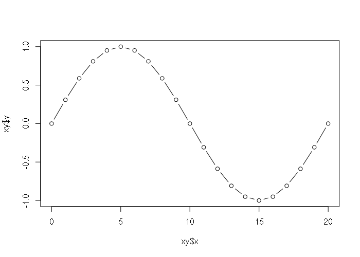
Lists can be passed to plotting functions if they have members named the same as the plotting function parameters.
> xy = list(x = 0:20, y = sin(pi * (0:20) / 10))
> plot(xy, type="b")
Access and Subsetting
List elements are accessed as slices or references.
List slices are sublists, and are specified with single square braces. The result is a list rather than an individual member.
> x = list("Alpha", "Beta", c("Gamma", "Delta"), list("Epsilon", 100))
> x[1]
[[1]]
[1] "Alpha"

> x[3:4]
[[1]]
[1] "Gamma" "Delta"

[[2]]
[[2]][[1]]
[1] "Epsilon"

[[2]][[2]]
[1] 100
To access or change the contents individual member of a list, you should use double square brackets.
> x = list("Alpha", "Beta", c("Gamma", "Delta"), list("Epsilon", 100))
> x[[1]]
[1] "Alpha"
> x[[1]] = "Omega"
> x[[1]]
[1] "Omega"
Members of lists can be named and accessed via those names, either with double square brackets or with the dollar sign operator.
> x = list(1, 2, "Joe", "Frank", 3.2)
> names(x) = c('ID', 'Party', 'Name', 'Mentor', 'Score')
> x
$ID
[1] 1

$Party
[1] 2

$Name
[1] "Joe"

$Mentor
[1] "Frank"

$Score
[1] 3.2

> x[['Name']]
[1] "Joe"
> x$Party
[1] 2
Appending and Deleting
To add elements to a list, you can set a member that doesn't exist (indexed by number or name), or use the c() function.
> x = list("Alpha", "Beta")
> x
[[1]]
[1] "Alpha"

[[2]]
[1] "Beta"
> x[length(x)] = "Omega"
> x['Season'] = "Spring"
> x = c("First", x)
> x
[[1]]
[1] "First"

[[2]]
[1] "Alpha"

[[3]]
[1] "Omega"

$Season
[1] "Spring"
You can delete elements by setting a slice of the list (single square brackets) to NULL:
> x = list("Alpha", "Beta", "Gamma")
> x[1:2] = NULL
> x
[[1]]
[1] "Gamma"
Operations
The lapply() function should be used if you need to perform an operation on every member of a list. Because lists are complex, mMathematical operations cannot be performed directly on members in the same manner as vectors or matrices.
> x = list(1, 3, 5, 8)

> x * 10
Error in x * 10 : non-numeric argument to binary operator

> lapply(x, function(z) z + 10)
[[1]]
[1] 11

[[2]]
[1] 13

[[3]]
[1] 15

[[4]]
[1] 18
Arrays and Matrices
Matrices are two-dimensional collections of a single data type. Arrays are collections of a single data type that can have any number of dimensions. Matrices are commonly used in complex mathematical operations.
Matrices and arrays are commonly output by functions as a componet of analysis. Notably, Matrices are used to represent pixels in images and raster GIS data.
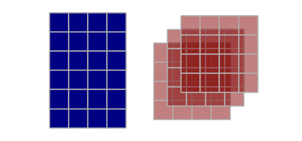
Creation
Matrices can be created directly from vectors of data using the matrix() function and specifying the number of rows and/or columns, and the order in which the data appears in the vector (byrow). Array creation with the array() function is similar, except the dimensions for each dimension is defined by the dim parameter, which is a vector with the lengths for each dimension.
> m = matrix(data = 1:12, ncol = 3, byrow = T)
> m
     [,1] [,2] [,3]
[1,]    1    2    3
[2,]    4    5    6
[3,]    7    8    9
[4,]   10   11   12
> m = matrix(data = 1:12, ncol = 3, byrow = F)
> m
     [,1] [,2] [,3]
[1,]    1    5    9
[2,]    2    6   10
[3,]    3    7   11
[4,]    4    8   12
> a = array(data = 1:12, dim = c(2,2,3))
> a
, , 1

     [,1] [,2]
[1,]    1    3
[2,]    2    4

, , 2

     [,1] [,2]
[1,]    5    7
[2,]    6    8

, , 3

     [,1] [,2]
[1,]    9   11
[2,]   10   12
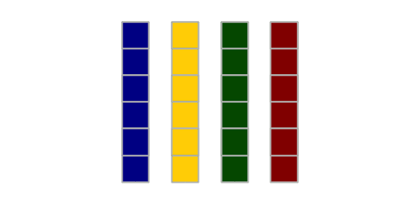
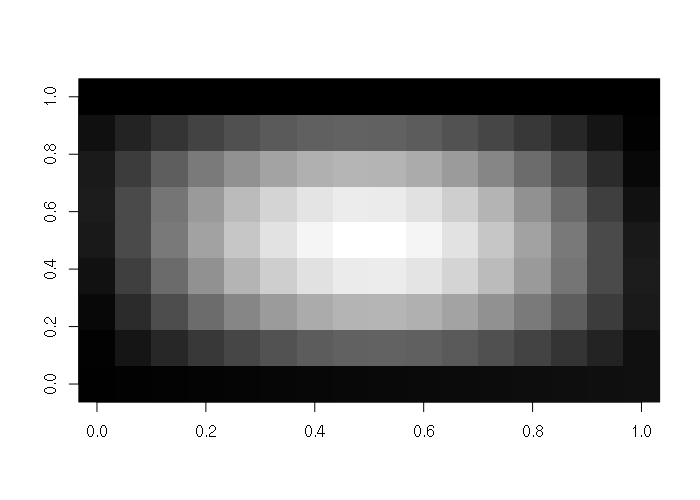
Visualization
Matrices can be visualized as 2-D colored surfaces using the image() function.
> x = as.matrix(read.csv("matrix-file.csv"))
> image(x, col=gray(seq(0,1,1/256)))
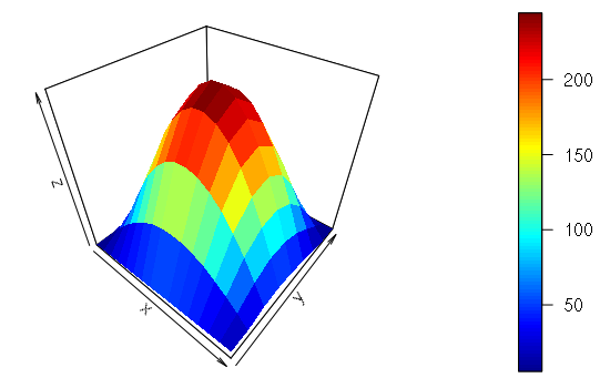
They can also be visualized as 3-D surfaces using the persp3D() function from the plot3D library.
> library(plot3D)
> x = as.matrix(read.csv("matrix-file.csv"))
> persp3D(z = x)
Import and Export
Matrices can be imported from CSV files by converting the output of read.csv() using the as.matrix() function. The file in the example below is HERE.
> x = as.matrix(read.csv("matrix-file.csv"))
> x
       X V1  V2  V3  V4  V5  V6 V7 V8
 [1,]  1  2   8  17  25  28  26 16  0
 [2,]  2 21  43  63  74  74  60 35  0
 [3,]  3 39  77 106 120 116  93 52  0
 [4,]  4 56 107 145 162 154 121 67  0
 [5,]  5 70 134 179 197 186 145 80  0
 [6,]  6 82 155 205 225 211 163 89  0
 [7,]  7 91 170 224 244 227 175 95  0
 [8,]  8 96 179 234 254 235 180 97  0
 [9,]  9 97 180 235 254 234 179 96  0
[10,] 10 95 175 227 244 224 170 91  0
[11,] 11 89 163 211 225 205 155 82  0
[12,] 12 80 145 186 197 179 134 70  0
[13,] 13 67 121 154 162 145 107 56  0
[14,] 14 52  93 116 120 106  77 39  0
[15,] 15 35  60  74  74  63  43 21  0
[16,] 16 16  26  28  25  17   8  2  0
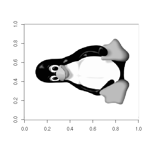
Matrices of pixels can also be read from a variety of image file formats. One lossless file format is the Portable Network Graphics (PNG) file. This PNG file in the example below is HERE.
> library(png)
> x = readPNG("tux-small-bw.png")
> class(x)
[1] "matrix"
> image(x, col=gray(seq(0,1,1/256)))
Access and Subsetting
Matrices can be accessed using square bracket array notation:
> m = as.matrix(read.csv("matrix-file.csv"))
> m
       X V1  V2  V3  V4  V5  V6 V7 V8
 [1,]  1  2   8  17  25  28  26 16  0
 [2,]  2 21  43  63  74  74  60 35  0
 [3,]  3 39  77 106 120 116  93 52  0
 [4,]  4 56 107 145 162 154 121 67  0
 [5,]  5 70 134 179 197 186 145 80  0
 [6,]  6 82 155 205 225 211 163 89  0
 [7,]  7 91 170 224 244 227 175 95  0
 [8,]  8 96 179 234 254 235 180 97  0
 [9,]  9 97 180 235 254 234 179 96  0
[10,] 10 95 175 227 244 224 170 91  0
[11,] 11 89 163 211 225 205 155 82  0
[12,] 12 80 145 186 197 179 134 70  0
[13,] 13 67 121 154 162 145 107 56  0
[14,] 14 52  93 116 120 106  77 39  0
[15,] 15 35  60  74  74  63  43 21  0
[16,] 16 16  26  28  25  17   8  2  0
> m[2,5]
V4
74
> m[1:4, 1:4]
     X V1  V2  V3
[1,] 1  2   8  17
[2,] 2 21  43  63
[3,] 3 39  77 106
[4,] 4 56 107 145
Appending and Deleting
Rows or columns can be appended to a matrix using the rbind() or cbind() functions, respectively.
Rows or columns can be deleted by setting the data frame to a subset of itself.
> m = matrix(1:16, ncol=4)
> m
     [,1] [,2] [,3] [,4]
[1,]    1    5    9   13
[2,]    2    6   10   14
[3,]    3    7   11   15
[4,]    4    8   12   16

> m = cbind(m, 101:104)
> m
     [,1] [,2] [,3] [,4] [,5]
[1,]    1    5    9   13  101
[2,]    2    6   10   14  102
[3,]    3    7   11   15  103
[4,]    4    8   12   16  104

> m = rbind(m, 201:205)
> m
     [,1] [,2] [,3] [,4] [,5]
[1,]    1    5    9   13  101
[2,]    2    6   10   14  102
[3,]    3    7   11   15  103
[4,]    4    8   12   16  104
[5,]  201  202  203  204  205

> m = m[2:4, 2:4]
> m
     [,1] [,2] [,3]
[1,]    6   10   14
[2,]    7   11   15
[3,]    8   12   16
Operations
Matrices and vectors can be used directly in mathematical operations:
> x = matrix(1:4, ncol=2)
> y = matrix(seq(10, 40, 10), ncol=2)

> x + 10
     [,1] [,2]
[1,]   11   13
[2,]   12   14

> x * 10
     [,1] [,2]
[1,]   10   30
[2,]   20   40

> x + y
     [,1] [,2]
[1,]   11   33
[2,]   22   44

> x * y
     [,1] [,2]
[1,]   10   90
[2,]   40  160
Note that these are direct element-by-element operations. Linear algebra matrix multiplication uses the %*% operator.
> x %*% y
     [,1] [,2]
[1,]   70  150
[2,]  100  220

> z = c(1000, 2000)
> x %*% z
      [,1]
[1,]  7000
[2,] 10000
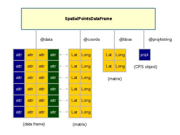
Spatial Objects
Objects in R are complex data structures that contain slots accessed with the @ operator. A slot can be any data type, including vectors, data frames or lists.
Objects are used with spatial data to keep all the disparate variables together in one collection. This practice of encapsulating data sets into complex structures that are dealt with as single entities is called object-oriented programming.
The slotNames() function displays the slots in an object. The SpatialPointsDataFrame object has the following slots:
> library(rgdal)
> data = read.csv("largest-us-cities.csv", as.is=T)
> cities = SpatialPointsDataFrame(data[,c("LONG","LAT")], data = data, proj4string = wgs84)
> slotNames(cities)
[1] "data"        "coords.nrs"  "coords"      "bbox"        "proj4string"
Creation
The sp library provides a set of related objects for representing the three fundamental geospatial vector data types: points, lines, polygons.
SpatialPointsDataFrame
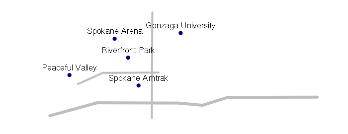
SpatialPointsDataFrame objects are used to represent sets of specific locations on the surface of the earth.
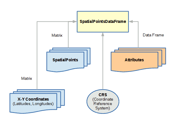
A spatial points object can be created with the SpatialPointsDataFrame() function, which minimally needs:
- A matrix of coordinates with longitude in the first column and latitude in the second
- A data frame of attributes associated with each coordinate pair
- A coordinate reference system (CRS) proj4 string that defines what coordinate system is used for longitude and latitude. The WGS 84 geographic coordinate system used by GPS is used in the example below
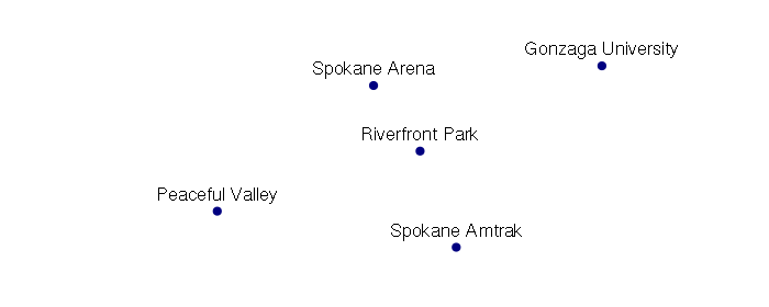
library(sp)
coords = matrix(data = c(
     -117.418692, 47.662245,
     -117.422896, 47.666241,
     -117.437009, 47.658582,
     -117.415427, 47.656382,
     -117.402272, 47.667440), ncol=2, byrow=T)

attributes = data.frame(name = c(
     'Riverfront Park',
     'Spokane Arena',
     'Peaceful Valley',
     'Spokane Amtrak',
     'Gonzaga University'), stringsAsFactors = F)

wgs84 = CRS("+proj=longlat +ellps=WGS84 +datum=WGS84 +no_defs")

points = SpatialPointsDataFrame(coords, data = attributes, proj4string = wgs84)
plot(points, pch=19, col="navy")
text(points@coords, labels = points$name, pos=3)
SpatialLinesDataFrame
SpatialLinesDataFrame objects are used to represent linear features like roads, streams, routes, etc.

main = matrix(byrow=T, ncol=2, data=c(
     -117.434318, 47.656684,
     -117.426615, 47.659040,
     -117.409202, 47.659105))

i90 = matrix(byrow=T, ncol=2, data=c(
     -117.379622, 47.653927,
     -117.387614, 47.653876,
     -117.395425, 47.652221,
     -117.403112, 47.652682,
     -117.428378, 47.652735,
     -117.443118, 47.650017))

division = matrix(byrow=T, ncol=2, data=c(
     -117.411288, 47.649558,
     -117.411121, 47.671755))

attributes = data.frame(
     name = c('Main Street', 'I-90', 'Division Street'),
     lanes = c(4, 6, 4))
lineslist = list(Lines(Line(main), ID=1),
     Lines(Line(i90), ID=2),
     Lines(Line(division), ID=3))

wgs84 = CRS("+proj=longlat +ellps=WGS84 +datum=WGS84 +no_defs")

streetlines = SpatialLines(lineslist, proj4string = wgs84)

streets = SpatialLinesDataFrame(streetlines, attributes)

plot(streets, col='gray', lwd=streets$lanes)
plot(points, pch=19, col='navy', add=T)
text(points@coords, labels = points$name, pos=3)
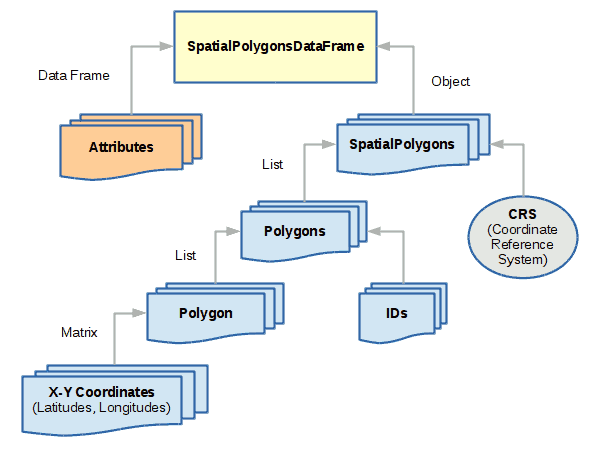
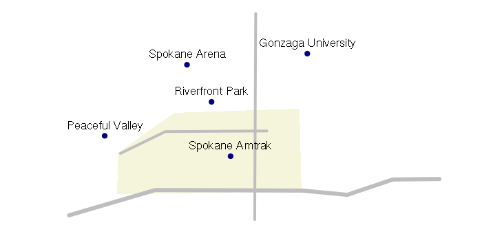
SpatialPolygonsDataFrame
SpatialPolygonsDataFrame objects are used to represent areas. While polygons
are simple collections of connected points, spatial polygons are
more complex because of the way areas relate to each other. For
example, an area like a state may be composed of multiple
land areas (like islands), and may contain holes (like water features).
coords = matrix(ncol=2, byrow=T, data=c(
     -117.434654, 47.656791,
     -117.425077, 47.661058,
     -117.403602, 47.661512,
     -117.403271, 47.652620,
     -117.434916, 47.652273))

attributes = data.frame(name='Downtown')

wgs84 = CRS("+proj=longlat +ellps=WGS84 +datum=WGS84 +no_defs")

polygon = Polygon(coords)
polygons = Polygons(list(polygon), ID=1)
sppolygons = SpatialPolygons(list(polygons), proj4string = wgs84)
downtown = SpatialPolygonsDataFrame(sppolygons, attributes)

plot(downtown, col='beige', border=NA, xlim=streets@bbox[1,], ylim=streets@bbox[2,])
plot(streets, col='gray', lwd=streets$lanes, add=T)
plot(points, pch=19, col='navy', add=T)
text(points@coords, labels = points$name, pos=3)
Import and Export
RGDAL
Spatial objects tend to be complex, and except for trivial cases, they are generally imported and exported to and from files rather than directly generated in R code.
Spatial points, lines and polygons can be imported from a number of different formats using the readOGR() function from the rgdal Geospatial Data Abstraction Library (GDAL/OGR).
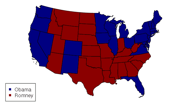
Shapefiles are an old geospatial data format introduced by ESRI in 1998, that still remains a least-common-denominator (safe) standard for distributing geospatial data to the general public.
The following example imports a shapefile of US state data and displays it as a choropleth with states colored by the winner of the 2012 presidential election. This data is available HERE.
library(rgdal)
states = readOGR('.', '2017-state-data')
states = states[!(states$ST %in% c('AK', 'HI')),]

color = ifelse(states$WIN2012 == 'Obama', 'navy', 'darkred')

usa_albers = CRS("+proj=aea +lat_1=20 +lat_2=60 +lat_0=40 +lon_0=-96 +x_0=0 +y_0=0
     +datum=NAD83 +units=m +no_defs")
states = spTransform(states, usa_albers)

plot(states, col=color)
legend('bottomleft', legend=c('Obama', 'Romney'), pch=15, col=c('navy', 'darkred'))
Projections
While the WGS 84 coordinate system used by GPS is perhaps the most common coordinate system, data from government sites will sometimes be in older coordinate systems, or coordinate systems (like one of the state plane coordinate systems) that are more-appropriate for the way that data is used by agencies and technicians in the field.
Maps are commonly created with layers of features overlaid on top of each other, and you should make sure that the coordinate systems match. The spTransform() function can be used to tranform data in one coordinate system to another.
Displaying geospatial data in WGS 84 tends to stretch distances horizontally the further you move from the equator. The US map above uses the coordinate system from the Albers Equal Area Conic projection so states display with approximately the same amount of area they actually have.
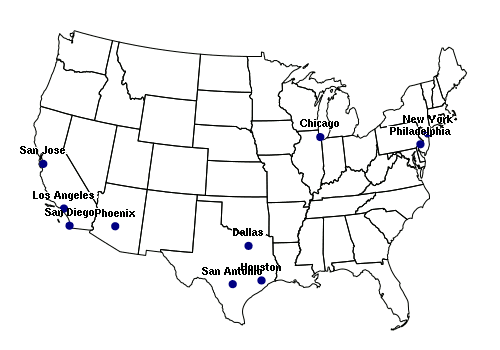
CSV Files of Points
Points can be imported from spreadsheet comma-separated variable (CSV) files. The CSV file used in the example below is available HERE.
library(rgdal)
data = read.csv("largest-us-cities.csv", as.is=T)
cities = SpatialPointsDataFrame(data[,c("LONG","LAT")], data = data, proj4string = wgs84)

usa_albers = CRS("+proj=aea +lat_1=20 +lat_2=60 +lat_0=40 +lon_0=-96 +x_0=0 +y_0=0
     +datum=NAD83 +units=m +no_defs")
cities = spTransform(cities, usa_albers)

states = readOGR('.', '2017-state-data')
states = states[!(states$ST %in% c('AK', 'HI')),]
states = spTransform(states, usa_albers)

plot(states)
plot(cities, pch=19, col="navy", add=T)
text(cities, labels=cities$NAME, pos=3, font=2, cex=0.8, col="white")
text(cities, labels=cities$NAME, pos=3, font=2, cex=0.7)
Access and Subsetting
Individual shapes in Spatial* objects can be accessed using square brackets in the same manner as a data frame, while leaving the second (column) dimension empty.
Although the attribute data frame of a Spatial* object is in the @data slot, the $ operator can be used directly with the name of the object to access attribute values.
You can get a list of the column names (attribute / field names) with the names() command.
> library(rgdal)
> states = readOGR('.', '2017-state-data')
> names(states)
 [1] "ST"         "State"      "WIN2012"    "DEM2012"    "PCDEM2012"
 [6] "GOP2012"    "PCGOP2012"  "WIN2016"    "DEM2016"    "PCDEM2016"
[11] "GOP2016"    "PCGOP2016"  "CHANGEDEM"  "CHANGEGOP"  "ELECTORAL"
[16] "PCELECTORA" "GOVERNOR"   "POP2014"    "PCPOP2014"  "WHITE2014"
[21] "PCWHITE"    "AREASQMI"   "POPSQMI"    "POP2010"    "URBAN2010"
[26] "RURAL2010"  "PCRURAL"
>
> states$GOVERNOR
 [1] DEM   GOP  GOP  GOP  GOP  GOP  GOP  DEM  GOP  GOP  DEM  DEM  DEM  DEM
[16] GOP  GOP  DEM  GOP  IND  GOP  GOP  DEM  GOP  DEM  DEM  GOP  GOP  GOP  GOP
[31] GOP  GOP  GOP  DEM  GOP  GOP  GOP  GOP  DEM  DEM  GOP  DEM  DEM  GOP  GOP
[46] DEM  DEM  GOP  GOP  DEM  GOP
Levels: DEM GOP IND
>
> par(mfcol=c(1,2))
> plot(states[states$ST == 'WA', ])
> plot(states[3:4,])
Appending and Deleting
New features can be added to a Spatial* object using the rbind() function, although the new features should have the exact same
Adding new columns to the attribute table is somewhat easier, although you will need to exercise caution to not affect the order of rows in the @data table and lose the relationship between the attributes and their respective shapes.
> library(rgdal)
> states = readOGR('.', '2017-state-data')
> states = states[!(states$ST %in% c('AK', 'HI')),]
> usa_albers = CRS('+proj=aea +lat_1=20 +lat_2=60 +lat_0=40 +lon_0=-96 +x_0=0 +y_0=0
+          +datum=NAD83 +units=m +no_defs')
> states = spTransform(states, usa_albers)
>
> states$POPRANK = order(states$POP2014)
> spplot(states, zcol='POPRANK')
> states$POPCHANGE = states$POP2014 - states$POP2010
> states$POPCHANGE
 [1] 812964  32013 560482 220103  31882  38115  31761  43905  67677 114224
[11]   5384  79736  39149 216228  69269 105260 946472 184107  37706 169499
[21]  31118 168384  58609  17956  29276  20906 214922  23876    174 109662
[31]  17048  16955  67500 101909  20528  94226 174583    887  11625  19126
[41]    685  37942  32334  56350    617  29828  61033   4599  82480
> spplot(states, zcol='POPCHANGE')
A far more common operation is an attribute join, where values from a related table are added to the attribute table based on a join key that associates them with the appropriate shape. Joins are performed with the merge() function from the sp library, which has a similar syntax to the merge() function in base R.
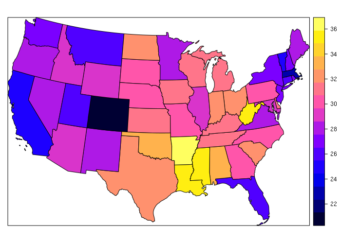
The example below merges obesity data with the state shapefile to create a choropleth.
> library(rgdal)
> states = readOGR('.', '2017-state-data', stringsAsFactors=F)
> states = states[!(states$ST %in% c('AK', 'HI')),]
> usa_albers = CRS('+proj=aea +lat_1=20 +lat_2=60 +lat_0=40 +lon_0=-96 +x_0=0 +y_0=0
+          +datum=NAD83 +units=m +no_defs')
> states = spTransform(states, usa_albers)
>
> st = c( 'AL', 'AK', 'AZ', 'AR', 'CA', 'CO', 'CT', 'DE', 'DC', 'FL', 'GA', 'HI',
+ 'ID', 'IL', 'IN', 'IA', 'KS', 'KY', 'LA', 'ME', 'MD', 'MA', 'MI', 'MN', 'MS',
+ 'MO', 'MT', 'NE', 'NV', 'NH', 'NJ', 'NM', 'NY', 'NC', 'ND', 'OH', 'OK', 'OR',
+ 'PA', 'RI', 'SC', 'SD', 'TN', 'TX', 'UT', 'VT', 'VA', 'WA', 'WV', 'WI', 'WY')
>
> obesity = c(33.5, 29.7, 28.9, 35.9, 24.7, 21.3, 26.3, 30.7, 21.7, 26.2, 30.5, 22.1, 28.9,
+ 29.3, 32.7, 30.9, 31.3, 31.6, 34.9, 28.2, 29.6, 23.3, 30.7, 27.6, 35.5, 30.2,
+ 26.4, 30.2, 27.7, 27.4, 26.9, 28.4, 27, 29.7, 32.2, 32.6, 33, 27.9, 30.2, 27,
+ 32.1, 29.8, 31.2, 31.9, 25.7, 24.8, 28.5, 27.3, 35.7, 31.2, 29.5)
>
> states = merge(states, data.frame(st, obesity), by.x = 'ST', by.y = 'st')
> spplot(states, zcol='obesity')
Visualization
Geospatial data is most commonly (but not always) visualized with maps, as shown in the examples above.
The plot() function is usually adequate for simple maps, as demonstrated above and below. A spplot() function is provided by the sp library to make quick thematic maps, although you can create more attractive maps using plot() and only a minimal number of additional functions and parameters.
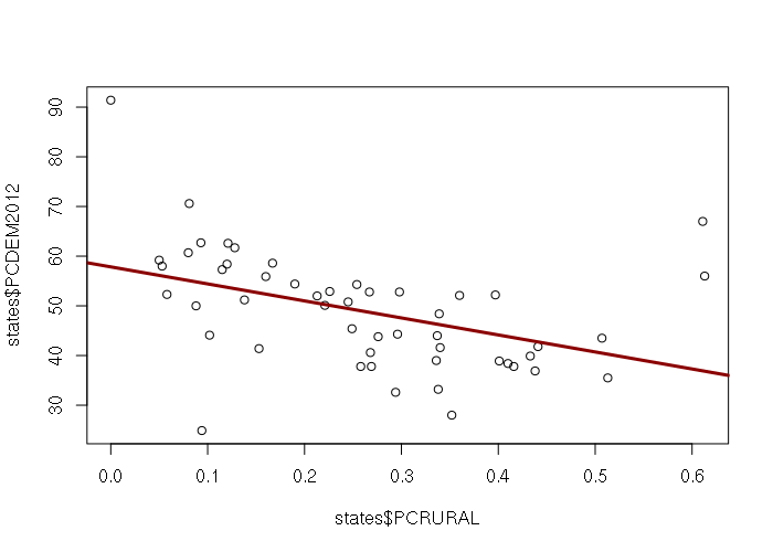
Attribute data is stored in the @data slot in the Spatial* objects and can be accessed with the $ operator, that data can be analyzed and visualized just like data in any other data frame. For example, the X-Y scatter plot below shows the inverse relationship by state between percentage of residents in rural areas and the percentage of the vote for President Obama in 2012. This data can be downloaded HERE.
> states = readOGR('.', '2017-state-data')
> plot(states$PCRURAL, states$PCGOP2012)
> m = lm(PCDEM2012 ~ PCRURAL, data=states)
> abline(m, lwd=3, col="darkred")
Spatial Raster Objects
The Raster* objects from the raster library are used to store raster geospatial data.
A raster is a (two-dimensional) matrix forming a regular grid of values over an area on the surface of the earth.
Rasters are commonly used with remotely-sensed data from satellites, which are usually images from various bands (frequencies) of light.
Full-color raster images need three overlapping raster layers representing red, green, and blue light frequencies, respectively.
Rasters can also be generated from aerial photography, or from point cloud data generated by aerial laser scanners (lidar).
Creation
A RasterLayer object is comprised of a single raster layer created with the raster() function.
A RasterStack is collection of multiple RasterLayer objects with the same spatial extent and resolution, created with the stack() function.
A RasterBrick is a multi-layer raster object created with the brick().
- RasterBricks are typically created from a single multi-band file, as opposed to a RasterStack created from separate files
- Processor time should be shorter if you can use a RasterBrick rather than a Raster Stack
- RasterBricks are less flexible than RasterStacks because all bands must be in a single file.
- If your bands are in separate files (as with Landsat data downloaded from EarthExplorer) you will use a RasterStack rather than a RasterBrick