Renewable Energy Analysis in R
This tutorial explores analysis and integration of renewable energy data from a variety of sources in R.
Energy Demand
The US Energy Information Administration (EIA) was created by the 1974 Federal Energy Administration (FEA) Act (P.L. 93-275, 15 USC 761) as a response to the early 1970s "energy crisis" and the need for additional Federal initiatives to collect, evaluate, analyze, and disseminate energy-related information. The Department of Energy Organization Act of 1977 created the United States Department of Energy by combining the Energy Research and Development Administration and the Federal Energy Administration, and making the EIA the primary federal energy statistics and analysis authority. (EIA 2021).
State Energy Profiles
EIA's State Energy Data System (SEDS) is a compilation of time series data on state energy production, consumption, prices, and expenditures. The objective is to provide data that is defined as consistently as possible over time and across sectors for analysis and forecasting purposes (EiA 2021).
A GeoJSON file of selected SEDS variables is available here.
library(sf)
states = st_read("2019-state-energy.geojson")
names(states)
[1] "ST" "Name"
[3] "GEOID" "AFFGEOID"
[5] "Square.Miles.Land" "Square.Miles.Water"
[7] "State.Name" "Population.MM"
[9] "Civilian.Labor.Force.MM" "GDP.B"
[11] "GDP.Per.Capita" "GDP.Manufacturing.MM"
[13] "Personal.Income.Per.Capita" "VMT.MM"
[15] "Farm.Land.MM.Acres" "Average.Temperature"
[17] "Precipitation.Annual" "Consumption.Coal.B.BTU"
[19] "Consumption.Jet.Fuel.B.BTU" "Consumption.Gasoline.B.BTU"
[21] "Consumption.Total.B.BTU" "Consumption.Per.Capita.MM.BTU"
[23] "Production.Coal.B.BTU" "Production.Gas.B.BTU"
[25] "Production.Oil.B.BTU" "Production.Renewable.B.BTU"
[27] "Production.Total.B.BTU" "Electricity.Interstate.Flow.GWH"
[29] "Electricity.Average.Cost" "Electricity.Consumption.GWH"
[31] "Electricity.Per.Capita.KWH" "Electricity.Hydro.GWH"
[33] "Electricity.Nuclear.GWH" "Electricity.Solar"
[35] "Electricity.Wind.GWH" "CO2.Total.MM.Tonnes"
[37] "CO2.Per.Capita.Tonnes" "Renewable.Standard.Type"
[39] "Renewable.Standard.Name" "Renewable.Standard.Year"
[41] "Senators.Party" "geometry"
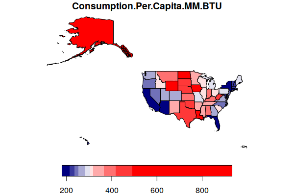
plot(states["Consumption.Per.Capita.MM.BTU"], breaks="quantile",
pal=colorRampPalette(c("navy", "white", "red")))
Energy Units
Government agencies in the USA commonly express energy supply and demand in British thermal units (BTU). One BTU is the amount of energy needed to raise the temperature of one pound of water by one degree (EIA 2021).
Because the BTU is a very small amount of energy, energy use by people and communities is commmonly expressed in millions, billions, or quadrillions (quads) of BTU.
In scientific literature, the more common international unit is the joule. There are around 1,055 joules in each BTU. For large-scale energy usage, the exajoule is a similar (but not exact) amount of energy as the quad.
In 2019, the 330 US residents consumed around 100.3 quadrillion BTU (quads) of total primary energy, or around 305.4 million BTU per person.
total_energy = sum(states$Consumption.Total.B.BTU, na.rm=T)

print(total_energy)

	[1] 100287202

total_population = sum(states$Population.MM, na.rm=T)

print(total_population)

	[1] 329.7

btu_per_capita = 1000 * total_energy / total population

print(btu_per_capita)

	[1] 304177137
Energy in Illinois
In 2019, Illinois consumed around 3.96 quadrillion BTU of total primary energy, or around 312.5 million BTU per person (EIA 2021a; EIA 2021b).
illinois = states[states$ST == "IL",]

print(100 * illinois$Consumption.Total.B.BTU / sum(states$Consumption.Total.B.BTU, na.rm=T))

	[1] 3.947184

illinois = st_transform(illinois, 4326)

print(illinois)

	bbox:           xmin: -91.51308 ymin: 36.9703 xmax: -87.49649 ymax: 42.50848
	epsg (SRID):    4269
	proj4string:    +proj=longlat +ellps=GRS80 +towgs84=0,0,0,0,0,0,0 +no_defs
	   ST     Name GEOID    AFFGEOID Square.Miles.Land Square.Miles.Water
	15 IL Illinois    17 0400000US17          55512.92           2400.229
	   State.Name Population.MM Civilian.Labor.Force.MM GDP.B GDP.Per.Capita
	15   Illinois          12.6                     6.1 897.1          71198
	   GDP.Manufacturing.MM Personal.Income.Per.Capita VMT.MM Farm.Land.MM.Acres
	15               108554                      62977 107525                 27
	   Average.Temperature Precipitation.Annual Consumption.Coal.B.BTU
	15                53.3                 41.9                 591909
	   Consumption.Jet.Fuel.B.BTU Consumption.Gasoline.B.BTU
	15                     189044                     557704
	   Consumption.Total.B.BTU Consumption.Per.Capita.MM.BTU Production.Coal.B.BTU
	15                 3958520                         312.5               1095887
	   Production.Gas.B.BTU Production.Oil.B.BTU Production.Renewable.B.BTU
	15                 2549                48045                     382793
	   Production.Total.B.BTU Electricity.Interstate.Flow.GWH
	15                2554925                         -372027
	   Electricity.Average.Cost Electricity.Consumption.GWH
	15                    28.25                      138319
	   Electricity.Per.Capita.KWH Electricity.Hydro.GWH Electricity.Nuclear.GWH
	15                      10920                   124                   98735
	   Electricity.Solar Electricity.Wind.GWH CO2.Total.MM.Tonnes
	15               251                14460               210.4
	   CO2.Per.Capita.Tonnes Renewable.Standard.Type      Renewable.Standard.Name
	15              16.69841               Mandatory Renewable Portfolio Standard
	   Renewable.Standard.Year Senators.Party                       geometry
	15                    2001     Democratic MULTIPOLYGON (((-91.51297 4...
Heat Rate
Because most current renewable energy technologies produce electricity rather than heat, in order to consider energy supply and demand in an electrified post-fossil-fuel future, we need a conversion factor to know how much electricity will be needed to satisfy future energy demand.
Assuming 100% efficiency, there are 3.412 BTU in each watt-hour of electricity. Dividing 2019 total primary energy consumption of 3,968,520 billion BTU by that conversion factor gives us 116,000 gigawatt-hours of electricity.
illinois$demand.gwh = illinois$Consumption.Total.B.BTU / 3.412

print(illinois$demand.gwh)
	[1] 1160176
Dividing by current electricity consumption (supplied largely by nuclear plants), we see that the renewable future will need an eight-fold increase in electrical generation.
illinois$demand.percent = 100 * illinois$demand.gwh / illinois$Electricity.Consumption.GWH

print(illinois$demand.percent)
	[1] 838.7682
However, because fossil fuel plants generally only convert about one-third of the heat energy in fuel to electrical energy, EIA uses a heat rate of 9.104 BTU per watt-hour (Davis et al. 2019 C-4). This same heat rate is used with renewables (solar and wind) to keep the numbers comparable across generating sources.
Using this conversion factor gives us a somewhat less daunting need to increase electrical generation by a factor of three.
illinois$demand.gwh = illinois$Consumption.Total.B.BTU / 9.104

print(illinois$demand.gwh)

	[1] 434811.1

illinois$demand.percent = 100 * illinois$demand.gwh / illinois$Electricity.Consumption.GWH

print(illinois$demand.percent)

	[1] 314.3538
Note that there are a number of gaps in this assessment:
- These number does not include energy needed to make products that are imported from other states and countries (embodied energy).
- These numbers do not consider industrial processes that use heat directly (like steelmaking), or technologies like airplane jet engines that currently have no clear pathway to electrification.
- These numbers assume an indefinite continuation of 2019 consumption practices that does not consider increases in demand due to population increases, or decreases in demand due to changes in technologies or lifestyles.
However, this kind of analysis gives us some general figures that can be used to assess the magnitude of the transformation and investment needed to move to a post-fossil-fuel world.
US Census Data
This tutorial will use US Census Bureau TIGER county area polygons and demographic data from the US Census Bureau's 2015-2019 American Community Survey 5-year estimates.
A GeoJSON file of that data is available here.
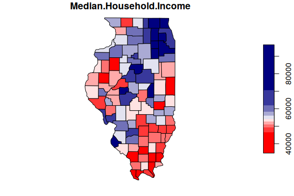
counties = st_read("2015-2019-acs-counties.geojson", quiet=T)

counties = counties[counties$ST == "IL",]

plot(counties["Median.Household.Income"], breaks="quantile",
	pal=colorRampPalette(c("red", "white", "navy")))
Wind Energy Potential
Another part of the response to the 1970s energy crises was the Solar Energy Research, Development, and Demonstration Act of 1974, which established the Solar Energy Research Institute, which opened in 1977. In 1991 the institute was designated a national laboratory of the US Department of Energy and renamed the National Renewable Energy Laboratory (NREL 2021).
NREL mission is to advance "the science and engineering of energy efficiency, sustainable transportation, and renewable power technologies and provides the knowledge to integrate and optimize energy systems" (NREL 2021). As part of their mission, NREL makes wide variety of data from their research activities available to the public.
Land-Based Wind Energy Supply Curves
NREL supply curve data is the result of assessment of renewable energy potential in terms of geographic, technical, and economic potential. Each aspect of this analysis adds a layer of complexity that is informed by related data and analysis. Factors include (NREL 2021):
- Environmental resource availability
- Land availability
- System design details
- Costs for site and transmission development.
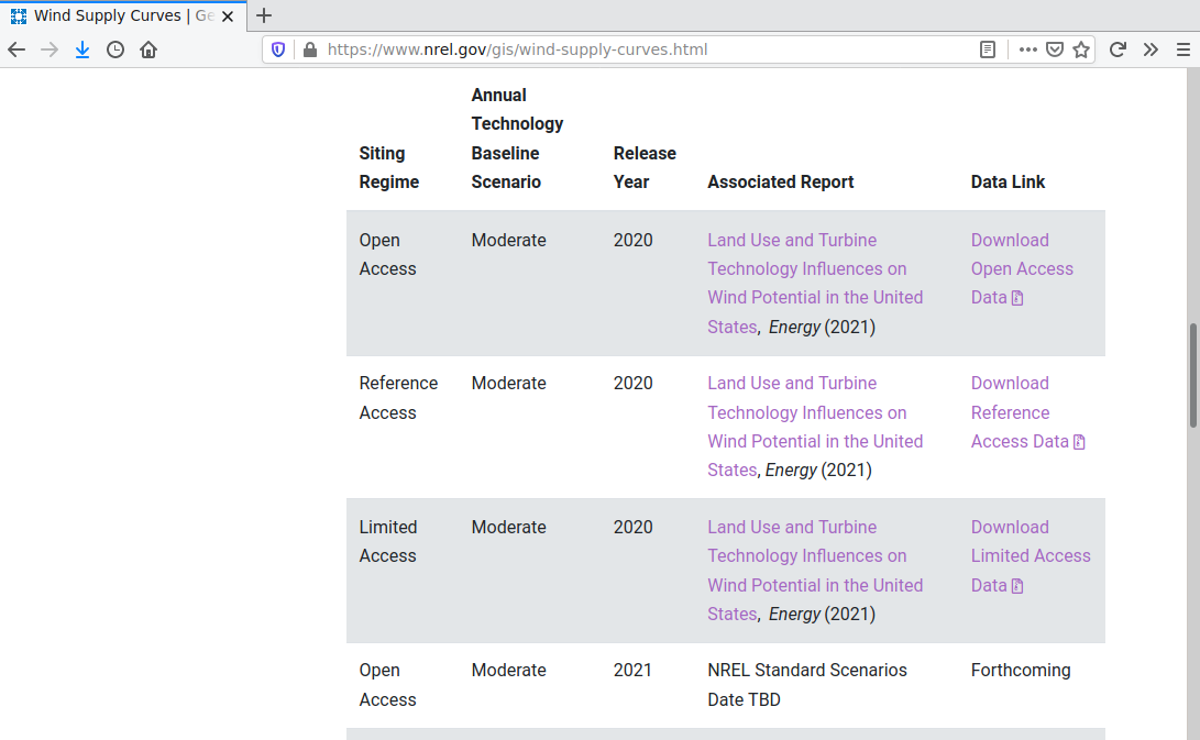
Supply curve data is made available in three collections that reflect different levels of that analysis (Lopez et al. 2021):
- Open Access: only applies land area exclusions based on physical constraints (e.g., wetlands, building footprints) or for protected lands
- Reference Access: incorporates a wider range of exclusions and is used by default in NREL's capacity expansion modeling
- Limited Access: applies the most restrictive land area exclusions
.zip files containing .csv files of supply curves can be downloaded from the NREL website.
Load the Supply Curve Data
The wind supply curve data is provided as a regular grid of points that can be loaded with the read.csv() function and converted to point features using the st_as_sf() function.
csv = read.csv("Reference_Access_Siting_Regime_ATB_Mid_Turbine.csv", as.is=T)

names(csv)

	[1] "X"                           "latitude"
	[3] "longitude"                   "area_sq_km"
	[5] "capacity_mw"                 "generation_mwh"
	[7] "capacity_factor"             "wind_speed_120meters"
	[9] "distance_to_transmission_km"

wind = st_as_sf(csv, coords=c("longitude", "latitude"), crs=4326)

plot(wind["capacity_factor"], breaks="quantile", pal=colorRampPalette(c("red", "white", "blue")))

Illinois Wind Supply Curve
The grid points within Illinois can be subset using the st_intersection() function.
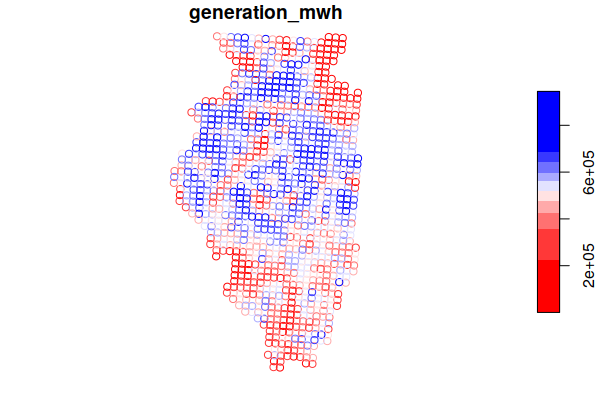
wind = st_intersection(wind, st_geometry(illinois))

plot(wind["generation_mwh"], breaks="quantile", pal=colorRampPalette(c("red", "white", "blue")))
The energy and power variables can be summed for each county by performing a spatial join using the aggregate() function.
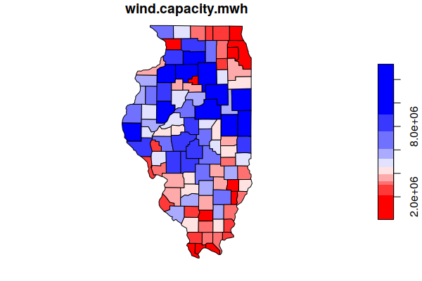
counties$wind.capacity.mwh = aggregate(wind["generation_mwh"], counties, FUN=sum)$generation_mwh

counties$wind.capacity.mw = aggregate(wind["capacity_mw"], counties, FUN=sum)$capacity_mw

plot(counties["wind.capacity.mwh"], breaks="quantile", pal=colorRampPalette(c("red", "white", "blue")))

counties = counties[order(counties$wind.capacity.mwh, decreasing=T),]

head(st_drop_geometry(counties[,c("Name", "wind.capacity.mwh")]))

		  Name wind.capacity.mwh
	633   Iroquois          13306549
	652     McLean          12965306
	648 Livingston          12877701
	647        Lee          11467672
	605  Champaign          10743495
	645    LaSalle          10549968
Wind Capacity Factor
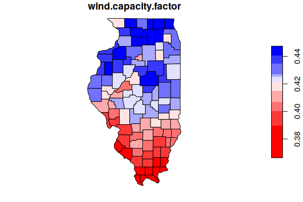
Capacity factor is the percentage of a wind turbine's nameplate capacity that it actually generates over time. Capacity factor is a function both of wind strength and consistency. Because there are few places where the wind blows strongly at all times, there will be periods where turbines are generating little or no electricity. Wind turbines are less economically feasable the lower the capacity factor.
counties$wind.capacity.factor = aggregate(wind["capacity_factor"], counties, FUN=mean)$capacity_factor

plot(counties["wind.capacity.factor"], breaks="quantile", pal=colorRampPalette(c("red", "white", "blue")))
Aggregate Wind Potential
Summing the potential wind megawatt-hours, converting to BTU, and then dividing by current state consumption indicates that wind power has the potential to supply all Illinois power needs.
illinois$wind.supply.mwh = sum(counties$wind.capacity.mwh, na.rm=T)

print(illinois$wind.supply.mwh)

	[1] 528758388

illinois$wind.supply.b.btu = illinois$wind.supply.mwh * 9.104 / 1000

print(illinois$wind.supply.b.btu)

	[1] 4813816

illinois$wind.supply.percent = 100 * illinois$wind.supply.b.btu /
	illinois$Consumption.Total.B.BTU

print(illinois$wind.supply.percent)

	[1] 121.6065
County Wind Potential
However, the wind power resource is unevenly distributed across the state relative to population. The heavily populated counties around St. Louis and Chicago have the most notable deficits in percent of demand that can be supplied with locally-generated wind power. This would necessitate construction of long-distance power lines to bring the wind power from sparsely-populated rural areas to the population centers.
counties$wind.capacity.b.btu = counties$wind.capacity.mwh * 9.104 / 1000

counties$demand.b.btu = counties$Total.Population *
	illinois$Consumption.Total.B.BTU /
	sum(counties$Total.Population, na.rm=T)

counties$wind.demand.percent = 100 * counties$wind.capacity.b.btu / counties$demand.b.btu

plot(counties["wind.demand.percent"], breaks="quantile",
	pal=colorRampPalette(c("red", "white", "blue")))
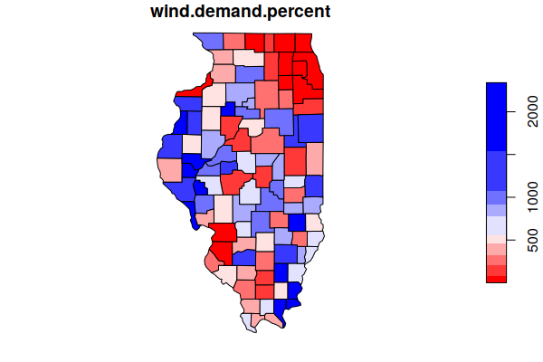
Ordering by percent makes it possible to list the top and bottom counties by local wind potential.
head(st_drop_geometry(counties[,c("Name", "wind.demand.percent")]))

		 Name wind.demand.percent
	631 Henderson            2339.703
	680  Schuyler            2261.218
	671      Pope            2197.794
	600     Brown            2137.698
	683     Stark            2038.666
	628  Hamilton            1901.108

 counties = counties[order(counties$wind.demand.percent, decreasing=F),]

 head(st_drop_geometry(counties[,c("Name", "wind.demand.percent")]))

	       Name wind.demand.percent
	611    Cook          0.07601945
	617  DuPage          0.20187488
	644    Lake          1.22054894
	694    Will         15.21790866
	640    Kane         16.77020079
	651 McHenry         28.64191445
Turbine Counts
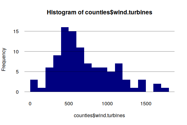
Although offshore wind turbines can have nameplate capacity of as much as six megawatts, the largest onshore turbines are 4 MW apiece, and the 2016 average was 2 MW apiece. (EIA 2017)
Dividing the maximum installed nameplate capacity by that average size gives us the number of turbines. The average number of turbines per county is 700, although the histogram shows that some counties would need over twice that number.
counties$wind.turbines = counties$wind.capacity.mw / 2

illinois$wind.turbines = sum(counties$wind.turbines, na.rm=T)

print(illinois$wind.turbines)

	[1] 71581.94

print(mean(counties$wind.turbines, na.rm=T))

	[1] 701.7837

hist(counties$wind.turbines, breaks=20,
	las=1, fg="white", col="navy", border=NA)

grid(nx=NA, ny=NULL, lty=1, col="#00000080")
Construction Cost
The 2019 average construction cost for wind turbines was $1,391 per kWh (EIA 2021).
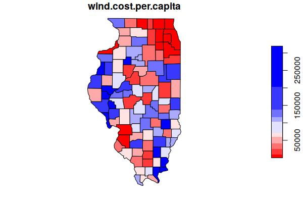
Multiplying that value times the number of turbines gives the estimated construction cost of $200 billion. A map of those expenditures per capita shows a significant amount of cash infusion into many rural counties. However, much of that cost would presumably be distributed to turbine manufacturers in other states or countries, and to specialized construction workers who would only stay in the county for a few years during construction.
cost.per.mw = 1391 * 1000

counties$wind.cost = counties$wind.capacity.mw * cost.per.mw

illinois$wind.cost = sum(counties$wind.cost, na.rm=T)

print(illinois$wind.cost)

	[1] 1.99141e+11

illinois$wind.cost.per.capita = illinois$wind.cost / (illinois$Population.MM * 1000000)

print(illinois$wind.cost.per.capita)

	[1] 15776.84

counties$wind.cost.per.capita = counties$wind.cost / counties$Total.Population

plot(counties["wind.cost.per.capita"], breaks="quantile",
	pal=colorRampPalette(c("red", "white", "blue")))

counties = counties[order(counties$wind.cost.per.capita, decreasing=T),]

head(st_drop_geometry(counties[,c("Name", "wind.cost.per.capita", "Total.Population")]))

		 Name wind.cost.per.capita Total.Population
	671      Pope             319467.7             4203
	680  Schuyler             292870.1             6953
	631 Henderson             289115.5             6809
	600     Brown             274755.4             6628
	628  Hamilton             258636.2             8176
	683     Stark             250838.3             5447
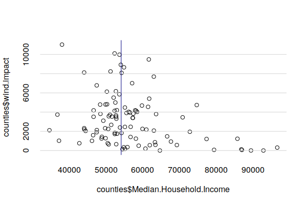
Operations and Maintenance Costs
In 2016 operations and maintenance costs for a wind farm was around $48,000 per MW (Reuters 2017).
Multiplying that times the wind capacity and dividing by population gives an estimate of per capita long-term local economic impact in each county.
counties$wind.om.cost = counties$wind.capacity.mw * 48000

counties$wind.impact = counties$wind.om.cost / counties$Total.Population

illinois$wind.om.cost = sum(counties$wind.om.cost, na.rm=T)

print(illinois$wind.om.cost)

	[1] 6859691202

illinois$wind.om.cost.per.capita = illinois$wind.om.cost / (illinois$Population.MM * 1000000)

print(illinois$wind.om.cost.per.capita)

	[1] 544.4199

illinois$median.household.income = median(counties$Median.Household.Income, na.rm=T)

plot(counties$Median.Household.Income, counties$wind.impact, fg="white", bty="n")

grid(nx=NA, ny=NULL, lty=1)

abline(v=illinois$median.household.income, col="navy")

counties = counties[order(counties$wind.impact, decreasing=T),]

head(st_drop_geometry(counties[,c("Name", "wind.impact", "Total.Population")]))

		 Name wind.impact Total.Population
	671      Pope   11024.048             4203
	680  Schuyler   10106.228             6953
	631 Henderson    9976.669             6809
	600     Brown    9481.136             6628
	628  Hamilton    8924.900             8176
	683     Stark    8655.814             5447
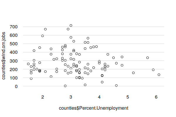
Operations and Maintenance Jobs
95 to 98% of jobs associated with wind farms are in the construction phase. However a significant number of technicians are needed to operate and maintain wind farms once construction is complete, although the exact number of direct and indirect jobs is highly variable across projects and countries. For the purposes of this analysis, we will use a Spanish figure of 0.2 direct operations and maintenence jobs per megawatt of installed capacity (Aldieri et al. 2019).
An estimated 28,600 maintainance and operations jobs would be created by a full deployment of wind turbines. However, plotting those jobs against long-term county unemployment rates indicates that those jobs would not necessarily be in the areas that most need them.
counties$wind.om.jobs = round(counties$wind.capacity.mw * 0.2)

illinois$wind.om.jobs = sum(counties$wind.om.jobs, na.rm=T)

print(illinois$wind.om.jobs)

	[1] 28633

plot(counties$Percent.Unemployment, counties$wind.om.jobs,
	las=1, fg="white", bty="n")

grid(nx=NA, ny=NULL, lty=1)

counties$Working.Age.Population = round(counties$Total.Population *
	(100 - counties$Percent.Under.18 - counties$Percent.65.Plus) / 100)

counties = counties[order(counties$wind.om.jobs, decreasing=T),]

head(st_drop_geometry(counties[,c("Name", "wind.om.jobs", "Working.Age.Population")]))

		  Name wind.om.jobs Working.Age.Population
	633   Iroquois          715                  15853
	648 Livingston          672                  21480
	652     McLean          671                 113384
	647        Lee          593                  21080
	605  Champaign          575                 144216
	645    LaSalle          565                  65732
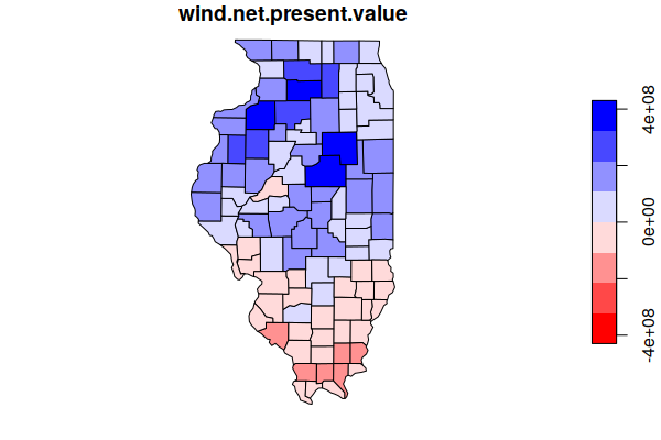
Net Present Value
Net present value (NPV) is a method for assessing the value of an investment based on the difference between expenditures and revenues over time. However, NPV is more than simple subtraction since it takes into account the time value of money over the lifetime of a capital investment. NPV can then be used to compare a potential investment with alternative investments. If the NPV of a project is negative, then the project should be avoided because it will lose money (Investopedia 2021).
For this calculation we assume the following:
- The wholesale price of electricity The 2020 average wholesale price of electricity was $34 per MWh, although prices varied widely depending on seasonal demand and fluctuations in supply, ranging from -$5 to $1750 per MWh (EIA 2021).
- This example uses $50 per MWh in order to place most counties in positive NPV.
- Wind turbine blades commonly last for 25 years (BBC 2020).
- We will use a common discount rate of 8%, which represents the annual cost of capital.
discount.rate = 0.08

turbine.life = 25

wholesale.price = 50

counties$wind.revenue = (counties$wind.capacity.mwh * wholesale.price) - counties$wind.om.cost

counties$wind.net.present.value = sapply(1:nrow(counties), function(index)
	((-counties$wind.cost[index] / (1 + discount.rate)) +
		+ sum(sapply(2:turbine.life, function(year)
			(counties$wind.revenue[index] / ((1 + discount.rate)^year))))))

limit = max(abs(range(counties$wind.net.present.value, na.rm=T)))

plot(counties["wind.net.present.value"], breaks = seq(-limit, limit, limit / 4),
	pal=colorRampPalette(c("red", "white", "blue")))

mean(counties$wind.net.present.value, na.rm=T)
	62323693
Installed Wind Capacity
The U.S. Wind Turbine Database
The EIA's United States Wind Turbine Database (USWTDB) provides the locations of land-based and offshore wind turbines in the United States, corresponding wind project information, and turbine technical specifications.
You can download the most recent update of the USWTDB from Download button on the EIA's US Energy Atlas page.
library(sf)
turbines = st_read("uswtdb_v4_1_20210721.geojson")
turbines = turbines[turbines$t_state == "IL",]
names(turbines)
[1] "case_id" "t_state" "p_name" "p_year" "p_tnum"
[6] "p_cap" "t_manu" "t_model" "t_cap" "t_hh"
[11] "t_rd" "t_rsa" "t_ttlh" "retrofit" "retrofit_y"
[16] "t_conf_atr" "t_conf_loc" "xlong" "ylat" "geometry"
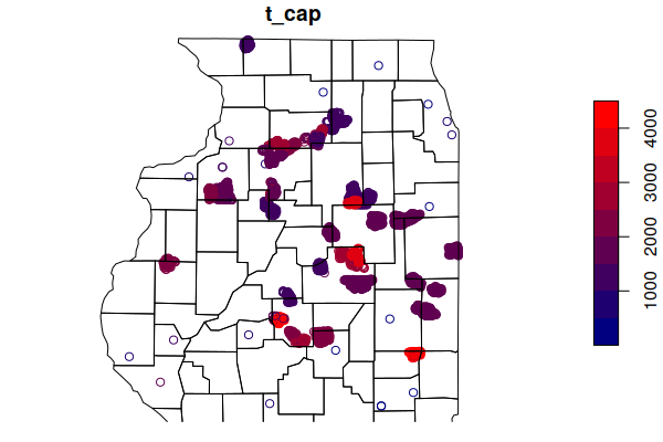
plot(turbines["t_cap"], pal=colorRampPalette(c("navy", "red")), reset=F)
plot(st_geometry(counties), add=T)
Current Percent of Potential
Given the total installed capacity from the USWTB and the potential capacity from the supply curve, we can determine the percent of potential capacity currently being tapped.
y = aggregate(turbines, counties, FUN=length)
counties$wind.installed.turbines = ifelse(is.finite(y$t_cap), y$t_cap, 0)
y = aggregate(turbines["t_cap"], counties, FUN=sum)
counties$wind.installed.mw = ifelse(is.finite(y$t_cap), y$t_cap / 1000, 0)
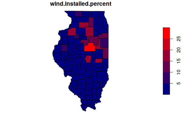
counties$wind.installed.percent = 100 * counties$wind.installed.mw / counties$wind.capacity.mw
plot(counties["wind.installed.percent"], pal=colorRampPalette(c("navy", "red")), reset=F)
We can get descriptive statistics of installation from the data.
illinois$wind.capacity.mw = sum(counties$wind.capacity.mw, na.rm=T)

print(illinois$wind.capacity.mw)

	[1] 143163.9

illinois$wind.installed.percent = 100 * sum(counties$wind.installed.mw, na.rm=T) /
	sum(counties$wind.capacity.mw, na.rm=T)

print(illinois$wind.installed.percent)

	[1] 3.521048

counties = counties[order(counties$wind.installed.percent, decreasing=T),]

head(st_drop_geometry(counties[,c("Name", "wind.installed.percent")]))

	       Name wind.installed.percent
	652  McLean               29.90932
	616 Douglas               19.36752
	647     Lee               18.97917
	632   Henry               18.47642
	653   Macon               18.28073
	645 LaSalle               18.13521
Solar Energy Potential
Solar Energy Supply Curves
Aside from wind and hydropower, solar power is the other major renewable energy source with an extensive body of proven technology, robust ongoing research, and immense potential.
As with wind, NREL provides gridded solar supply curve data which can be downloaded from their website..
csv = read.csv("pv_reference_2020.csv", as.is=T)

names(csv)

	[1] "sc_gid"                       "capacity_factor"
	[3] "global_horizontal_irradiance" "capacity_mw"
	[5] "area_sq_km"                   "latitude"
	[7] "longitude"                    "distance_to_transmission_km"

solar = st_as_sf(csv, coords=c("longitude", "latitude"), crs=4326)

plot(solar["capacity_factor"], breaks="quantile", pal=colorRampPalette(c("blue", "white", "red")))
Illinois Solar Energy Supply Curves
Subsetting to the state of Illinois, we see an expected distribtion in capacity factor, although the variance is small.
solar = st_intersection(solar, st_geometry(illinois))

plot(solar["capacity_factor"], breaks="quantile", pal=colorRampPalette(c("blue", "white", "red")))
The supply curve data does not include a potential annual generation figure, although one can be calculated from the capacity factor and potential capacity in MW.
solar$generation_mwh = solar$capacity_mw * solar$capacity_factor * 24 * 365

plot(solar["generation_mwh"], breaks="quantile", pal=colorRampPalette(c("blue", "white", "red")))
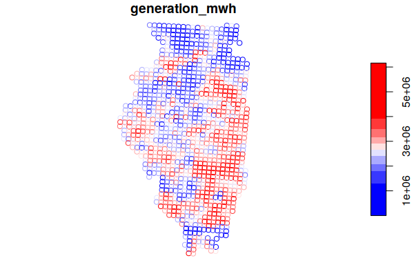
County Solar Energy Supply Curves
The energy and power variables can be summed for each county by performing a spatial join using the aggregate() function.
counties$solar.capacity.mwh = aggregate(solar["generation_mwh"], counties, FUN=sum)$generation_mwh
counties$solar.capacity.mw = aggregate(solar["capacity_mw"], counties, FUN=sum)$capacity_mw
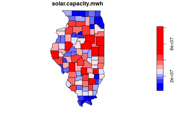
plot(counties["solar.capacity.mwh"], breaks="quantile",
pal=colorRampPalette(c("blue", "white", "red")))
counties = counties[order(counties$solar.capacity.mwh, decreasing=T),]
head(st_drop_geometry(counties[,c("Name", "solar.capacity.mwh")]))
Name solar.capacity.mwh
652 McLean 51501691
616 Douglas 24894366
647 Lee 40256446
632 Henry 45069415
653 Macon 36563448
645 LaSalle 44270513
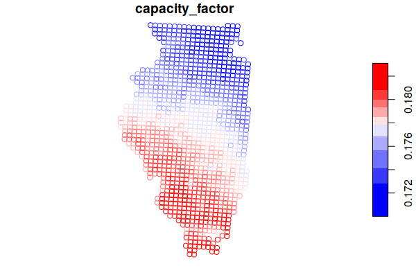
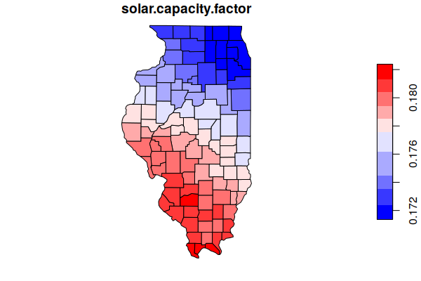
Solar Capacity Factor
Capacity factor is the percentage of a solar panel's nameplate capacity that it actually generates over time. Capacity factor is a function both of solar irradience and cloud cover.
counties$solar.capacity.factor = aggregate(solar["capacity_factor"], counties, FUN=mean)$capacity_factor

plot(counties["solar.capacity.factor"], breaks="jenks", pal=colorRampPalette(c("blue", "white", "red")))
Aggregate Solar Potential
Summing the potential solar megawatt-hours, converting to BTU, and then dividing by current state consumption indicates that solar power has the potential to supply all Illinois power needs.
illinois$solar.capacity.factor = mean(solar$capacity_factor, na.rm=T)

print(illinois$solar.capacity.factor)

	[1] 0.1772521

illinois$solar.capacity.mwh = sum(counties$solar.capacity.mwh, na.rm=T)

print(illinois$solar.capacity.mwh)

	[1] 2834465381

illinois$solar.capacity.b.btu = illinois$solar.capacity.mwh * 9.104 / 1000

print(illinois$solar.capacity.b.btu)

	[1] 25804973

illinois$solar.capacity.percent = 100 * illinois$solar.capacity.b.btu /
	illinois$Consumption.Total.B.BTU

print(illinois$solar.capacity.percent)

	[1] 651.8844
Rooftop Installations
Unlike wind turbines that can be placed above farm fields or pasture with limited effect on use of the land for other purposes, solar panels require surface area that blocks the sun and is much more intrusive.
One common location for solar panel installation is on the roofs of buildings, especially single family homes. While residential rooftop installations are often considered unattractive and can run afoul of homeowners associations, they are nonetheless a source of surface area that does not directly interfere with the use of the land for residential purposes.
Estimation of potential surface area for solar panel installation is an area of extensive past and ongoing research. However, most methodologies require detailed building data and / or interpretation of remotely sensed data (Groppi et al. 2018).
As a rough estimate, we will use a simple model based on the following assumptions:
- Home ownership in Illinois is primarily associated with single-family rather than multi-family housing.
- The number of households times the percent of home owners gives the potential number of residential rooftop solar installations.
- An arbitrary 50% of rooftops are assumed to be unavailable either because of size, orientation, vegetation, or NIMBY.
- A typical residential solar installation is 8.2 kW, with a $24,400 total installation cost (Etheridge 2019).
counties$solar.rooftops = counties$Total.Households * counties$Percent.Homeowners / 100 * 0.5

illinois$solar.rooftops = sum(counties$solar.rooftops, na.rm=T)

print(illinois$solar.rooftops)

	[1] 1601280

counties$solar.rooftops.cost = counties$solar.rooftops * 24400

illinois$solar.rooftops.cost = sum(counties$solar.rooftops.cost, na.rm=T)

print(illinois$solar.rooftops.cost)

	[1] 39071236319

counties$solar.rooftops.mw = counties$solar.rooftops * 8.2 / 1000

illinois$solar.rooftops.mw = sum(counties$solar.rooftops.mw, na.rm=T)

print(illinois$solar.rooftops.mw)

	[1] 13130.5

counties$solar.rooftops.mwh = counties$solar.rooftops.mw * counties$solar.capacity.factor * 365 * 24

counties$solar.rooftops.b.btu = counties$solar.rooftops.mwh * 9.104 / 1000

illinois$solar.rooftops.b.btu = sum(counties$solar.rooftops.b.btu, na.rm=T)

print(illinois$solar.rooftops.b.btu)

	[1] 182126
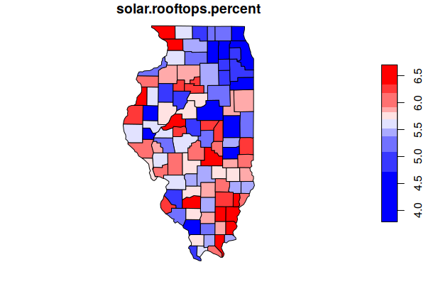
Solar Rooftop Demand Percentage
When restricting solar installation to the fairly small amount of area represented by rooftops, the percentage of demand that can be satisfied by solar drops significantly from the generous estimates in the NREL solar supply curve data.
counties$demand.b.btu = counties$Total.Population *  illinois$Consumption.Total.B.BTU /
	sum(counties$Total.Population, na.rm=T)

counties$solar.rooftops.percent = 100 * counties$solar.rooftops.b.btu / counties$demand.b.btu

plot(counties["solar.rooftops.percent"], breaks="quantile", pal=colorRampPalette(c("blue", "white", "red")))

illinois$solar.rooftops.percent = 100 * sum(counties$solar.rooftops.b.btu, na.rm=T) /
		sum(counties$demand.b.btu, na.rm=T)

print(illinois$solar.rooftops.percent)

	[1] 4.600692
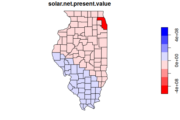
Net Present Value
As with wind, we can use net present value (NPV) to evaluate the cost effectiveness of solar across Illinois.
For this calculation we assume the following:
- Although the mean wholesale price of electricity in 2020 was $34 per MWh (EIA 2021), the high capital cost of solar will yield a highly negative NPV at that price in Illinois. For this example we use a significantly higher price of $180 that dramatizes how expensive energy would need to be to make solar cost effective in Illinois.
- Solar panels are typically warrantied for 20 - 25 years. Assuming the structures holding the panels are not damaged, the panels will continue to work, although their output degrades around 0.5% per year to around 90% percent by year 20 (NREL 2021).
- We assume no significant operations and maintenance cost and assume any cleaning will be performed by the homeowner as sweat equity.
- We will use a common discount rate of 8%, which represents the annual cost of capital.
discount.rate = 0.08

panel.life = 25

wholesale.price = 190

counties$solar.rooftops.revenue = counties$solar.rooftops.mwh * wholesale.price

counties$solar.net.present.value = sapply(1:nrow(counties), function(index)
	((-counties$solar.rooftops.cost[index] / (1 + discount.rate)) +
		+ sum(sapply(2:panel.life, function(year)
			(counties$solar.rooftops.revenue[index] / ((1 + discount.rate)^year))))))

limit = max(abs(range(counties$solar.net.present.value, na.rm=T)))

plot(counties["solar.net.present.value"], breaks = seq(-limit, limit, limit / 4),
	pal=colorRampPalette(c("red", "white", "blue")))

mean(counties$solar.net.present.value, na.rm=T)

	[1] 8593710
Intermittency
Intermittency with renewable energy sources means that they are not always available. While all generating facilities need occasional downtime for maintenance, solar and wind have significant daily and seasonal periods where they generate little or no power because the sun is not shining or the wind is not blowing.
However, energy demand in an industrialized society involves a constant base load with additional cycles and surges that rise above base load in response to environmental or social conditions (such as hot summer afternoons).
There are numerous ways to address intermittency:
- Interconnection: Electricity is distributed in a grid that interconnects users and generating plants. When wind is not blowing in one area, it may be blowing in another, and the surplus energy can flow through the grid to compensate for low output from another facility.
- Complimentary sources: Wind power tends to drop in the summer while solar output increases. Using complimentary sources like this can smooth out intermittent dips.
- Demand management and pricing: Grid operators can increase energy prices when demand begins to near supply limits. This can encourage optional users to reduce energy use until supply improves and prices drop. This can also encourage countercyclical use of energy, such as charging electric vehicles at night when electricity demand is often lower than during the day.
- Peaker plants: Small, distributed natural gas or diesel plants that are easy to start and stop can be added to the grid at times of peak demand.
- Batteries: Large banks of batteries can be used to store surplus power and send it back to the grid when generation is less than demand.
- Pumped storage: These are hydraulic batteries. Reservoirs can be filled with water when demand is low, and then drained through generators when backup power is needed in a manner similar to hydroelectric dams. The primary challenge with pumped storage is the limited number of suitable, available locations.
- Conservation: Reducing short-term or long-term demand with changes in technology or lifestyles can shift the supply/demand balance so that intermittency is less of an issue.
Energy Cycles
In order get get some sense of the amount of storage that might be needed for an Illinois powered entirely by renewables, we need fine-grained information on resource availability so we can find the peak amount of power that must be stored to provide 100% reliability to energy users.
Renewables.ninja is an unfortunately named web app created by energy researchers Iain Staffell and Stefan Pfenninger that allows you to find daily and monthly capacity factors for both solar and wind at specific locations on the surface of the earth.
The source data for Staffella and Pfenninger's models is The Modern-Era Retrospective analysis for Research and Applications, Version 2 (MERRA-2), from the Global Modeling and Assimilation Office at NASA's Goddard Space Flight Center. This dataset is a global atmospheric reanalysis that uses satellite observations since the 1980s to create a time series of grids of atmospheric and land surface conditions (NCAR 2021; Gelaro et al. 2017). This data is interpreted by the Staffell and Pfenninger's web app to estimate hourly wind and solar availability across an entire year (Pfenninger and Staffell 2016; Staffell and Pfenninger 2016).
The video below demonstrates how to download data from Renewables.ninja.
Hourly Data
Load the wind time series into a data frame.
csv = read.csv("ninja_wind_40.1347_-88.1976_uncorrected.csv", as.is=T, skip=3)

names(csv)

	[1] "time"        "local_time"  "electricity" "wind_speed"

storage = csv[,c("local_time", "electricity")]

names(storage) = c("local_time", "wind")

storage$wind = csv$electricity

csv = read.csv("ninja_pv_40.1347_-88.1976_uncorrected.csv", as.is=T, skip=3)

names(csv)

	[1] "time"               "local_time"         "electricity"
	[4] "irradiance_direct"  "irradiance_diffuse" "temperature"

storage$solar = csv$electricity
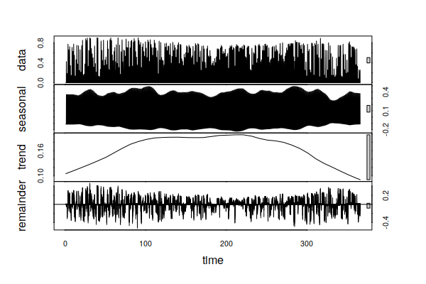
Time Series Decomposition
Using the xts() function to create a time series and using stl() function to decompose the wind time series into seasonal, trend, and random components shows a noticeable dip in capacity factor during the summer.
library(xts)

storage.series = xts(storage[,c("wind", "solar")], as.POSIXlt(storage$local_time))

attr(storage.series, "frequency") = 24

decomposition = stl(as.ts(storage.series$wind), s.window=24, t.window=2400)

plot(decomposition)

In the opposite of wind energy, the time series decomposition of solar shows a noticeable peak during the summer.
decomposition = stl(as.ts(storage.series$solar), s.window=24, t.window=2400)

plot(decomposition)
Batteries
One mitigation measure currently being actively developed and deployed is battery storage. Batteries are charged when there is surplus supply available, and those batteries then fill the gap when demand exceeds supply.
The primary challenge with batteries as of this writing is their expense. In 2018, utility-scale battery storage averaged around $625 per kilowatt hour (EIA 2020). Although costs can run as low as $175 per kWh, Ziegler et al. (2019) estimated costs would need to drop to $20 per kWh to be competitive with 2019 power sources.
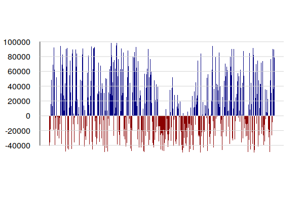
In the simulation below, we assume a demand base load that evenly distributes total energy use across the year 24/7/365.
The bar plot shows the balance of supply and demand with blue bars on top representing surplus generation and red bars on the bottom representing unmet base load demand.
storage$demand.mw = illinois$demand.gwh * 1000 / 365 / 24

storage$solar.mw = illinois$solar.rooftops.mw * storage$solar

storage$wind.mw = sum(counties$wind.capacity.mw, na.rm=T) * storage$wind

storage$balance = storage$solar.mw + storage$wind.mw - storage$demand.mw

barplot(storage$balance, col=ifelse(storage$balance > 0, "navy", "darkred"), border=NA, las=1, space=0, tck=0)

grid(nx=NA, ny=NULL, lty=1)
Iterative Storage Model
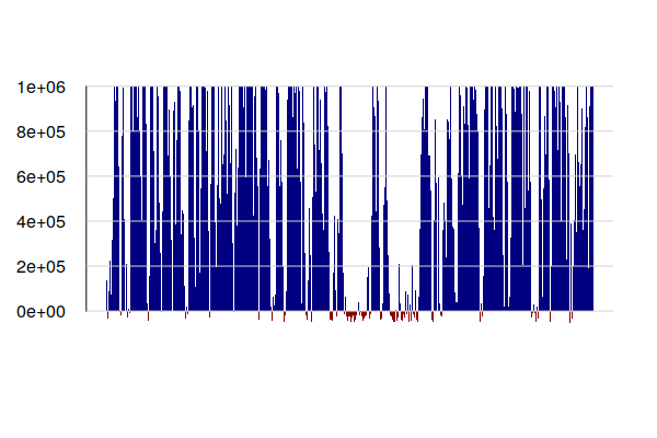
Adding storage to the simulation, the for() loop in this model proceeds iteratively through each hour of the year.
The overall battery capacity (in MWh) below is chosen to balance cost and unmet demand. You can modify the variable to test other possibilities.
- If the energy balance is positive (more generation than demand), the surplus energy is added to storage up to the limit of the battery capacity.
- If the energy balance is negative, but adequate storage is available to make up that deficit, it is taken from the battery.
- Otherwise, there is inadequate battery energy to make up the deficit. Whatever energy is available in the battery is drained to zero and the deficit is flagged.
The bar plot shows the level of battery charge on the top blue bars, and unmet demand on the bottom red bars.
storage$level = 0

storage$deficit = 0

battery.capacity = 1000000

for (x in 2:nrow(storage)) {
	if (storage$balance[x] >= 0) {
		storage$level[x] = min(storage$level[x - 1] + storage$balance[x], battery.capacity)
		storage$deficit[x] = 0
	} else if (storage$level[x - 1] >= -storage$balance[x]) {
		storage$level[x] = storage$level[x - 1] + storage$balance[x]
		storage$deficit[x] = 0
	} else {
		storage$deficit[x] = storage$balance[x] - storage$level[x - 1]
		storage$level[x] = 0
	}
}

barplot(t(storage[,c("level", "deficit")]), col=c("navy", "darkred"), border=NA, las=1, space=0, tck=0)

grid(nx=NA, ny=NULL, lty=1)
Given the wide range of costs per MWh of storage given above, we can get a range of the cost for the the battery storage modeled above.
illinois$battery.cost = list(battery.capacity * c(20, 175, 625))

print(illinois$battery.cost)

[[1]]
[1] 2.00e+07 1.75e+08 6.25e+08
Saving Your Analysis
The three core analytical objects can be saved as .rds files so you can use them again later without having to completely re-run your analysis.
saveRDS(illinois, "2021-illinois-state-analysis.rds")
saveRDS(counties, "2021-illinois-county-analysis.rds")
saveRDS(storage, "2021-illinois-storage-analysis.rds")
They can be reloaded with the readRDS() function.
illinois = readRDS("2021-illinois-state-analysis.rds")
counties = readRDS("2021-illinois-county-analysis.rds")
storage = readRDS("2021-illinois-storage-analysis.rds")