Creating a Point Map From a CSV File in R

This tutorial demonstrates how to create a variety of point maps in R from CSV files.

The CSV file for these examples is a list of houses of worship in Farmingdale, NY that is available here.

Single Symbol Point Map

These examples use the Simple Features (sf) library. While you may see examples on the web that use the older sp library, the sf library is easier to use and is recommended over sp.

read.csv() the CSV file into a data frame.
Use st_as_sf() to create simple features from the data frame using the lat/long coordinates.
- The crs=4326 parameter specifies that the coordinates are WGS 1984 latitudes and longitudes (EPSG 4326).
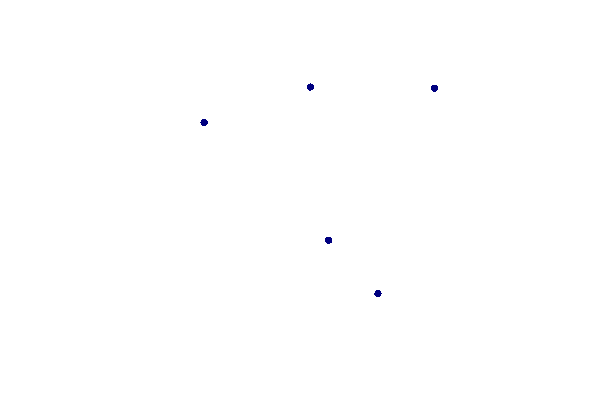
plot() the points.
- We plot the st_geometry() of the points so that plot() draws all features the same without considering any of the attributes.
- The pch parameter specifies the character to be drawn (a circle).
- The col parameter specifies the color for the circles.

library(sf)

data = read.csv("2018-farmingdale-bethpage-worship.csv", as.is=T)

points = st_as_sf(data, coords = c("Longitude", "Latitude"), crs = 4326)

plot(st_geometry(points), pch=16, col="navy")

Optionally, you can use st_write() to save the features as a GeoJSON file for later use.

st_write(points, dsn="2018-farmingdale-bethpage-worship.geojson", delete_dsn=T)

Base Map

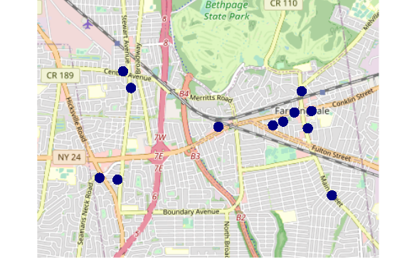
Since points by themselves usually don't give much context for where they are located, it may be helpful to plot them over an OpenStreetMap base map using OpenStreetMap library functions.

Get the map tiles with the openmap() function.
- The upperLeft and lowerRight parameters are lat/long coordinates to define the area to be mapped.
- The type parameter specifies the source for the map tiles. osm specifies OpenStreetMap, which is reliable.
- This can take awhile to load the tiles.
You will need to plot() the base map first so it is under any features plotted on top of it.
Because the osm map is in a spherical Mercator projection, you need to st_transform() the features into that coordinate system.
You can then plot() the points.
- The cex parameter specifies a multiplication factor to scale the points.
- add=T is needed so the plot adds the points to the map rather than redrawing the entire plot.

Sys.setenv(NOAWT=1)

library(OpenStreetMap)

upperLeft = c(40.75, -73.50)

lowerRight = c(40.71, -73.43)

base_map  = openmap(upperLeft, lowerRight, type="osm")

plot(base_map)

points = st_transform(points, osm())

plot(st_geometry(points), pch=16, col="navy", cex=2, add=T)

The Sys.setenv(NOAWT=1) call indicates that the OpenStreetMap package should not use the java.awt Abstract Window Toolkit classes for creating user interfaces and for painting graphics and images, since a display may not be available if you are using the OpenStreetMap library on a server installation of R Studio. This should address the java.awt.AWTError: Can't connect to X11 window server using ':0' as the value of the DISPLAY variable error. You will need to Restart R if you have already loaded OpenStreetMap before adding this line to your code.

Labels

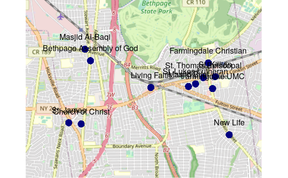
Labels can be added with the text() function.

Labeling presents a challenge with R base graphics because there is no facility for handling collisions.

This could be handled by manually adding pos and offset values to the spreadsheet to move the labels off of each other. But the simpler solution is to just avoid labels if possible.

plot(base_map)

points = st_transform(points, osm())

plot(st_geometry(points), pch=16, col="navy", cex=2, add=T)

text(st_coordinates(points), labels=points$Church, pos=3, offset=1)

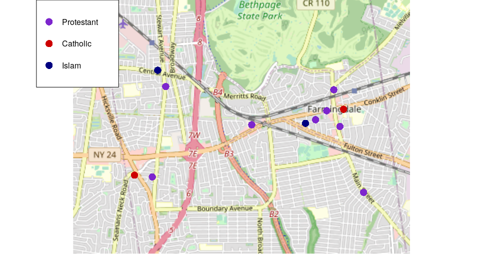
Categorical Maps

You can plot points colored by a categorical variable.

Create a vector of desired colors. Methods for specifying colors including a list of color names is here.
You should avoid choosing colors that require readers to distinguish between red and green, since around 8% of men and 0.5% of women have red-green color blindness (NIH 2020).
Set the the vector element names() to the unique() categories.
plot() the base map and the points with the palette vector indexed by the category field.
Provide a legend() so it is clear what the colors mean.

palette = c("purple3", "red3", "navy")

names(palette) = unique(points$Tradition)

plot(base_map)

plot(st_geometry(points), pch=16, col=palette[points$Tradition], cex=2, add=T)

legend("topleft", legend=names(palette), col=palette, 
	pch=16, pt.cex=2, title="Capacity")

Map of houses of worship in Farmingdale, NY by religious tradition

Bubble Maps

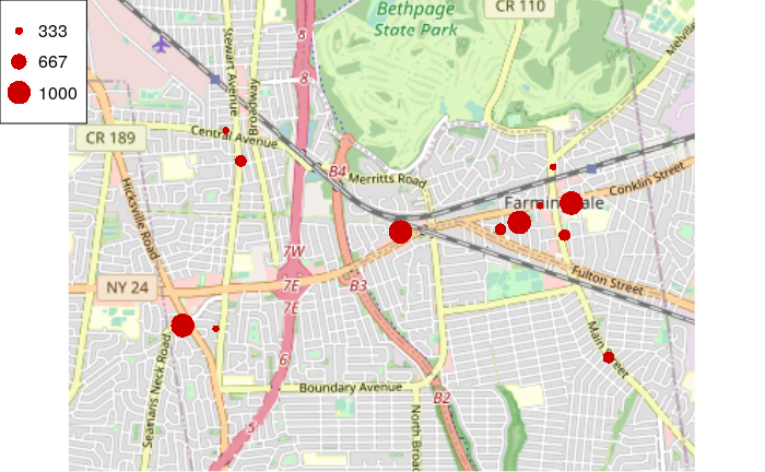
You can use the cex plot() parameter to vary the size of symbols by a quantiative variable.

plot(base_map)

scaling = 3 * points$Capacity / max(points$Capacity)

plot(st_geometry(points), pch=16, col="red3", cex=scaling, add=T)

steps = round(seq(1,3,1) * max(points$Capacity) / 3)

legend("topleft", legend=steps, col="red3", pch=16, pt.cex=1:3)

Seating capacity of houses of worship in Farmingdale, New York in 2018

Bivariate Maps

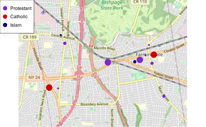
You can map both variables by varying both color and size.

plot(base_map)

plot(st_geometry(points), pch=16, col=palette[points$Tradition], cex=scaling, add=T)

legend("topleft", legend=names(palette), col=palette, pch=16, pt.cex=2)

Interactive Leaflet Maps

Leaflet is a popular and easy-to-use open-source JavaScript library for creating interactive maps.

The Leaflet library for R can be used to create interactive maps in notebooks.

Leaflet chunks will cause knit to a Word or PDF document to fail because paper documents cannot contain interactive maps. If you need to knit a notebook with a Leaflet chunk, you need to comment out the Leaflet code or temporarily remove the chunk while knitting the document and replacing the chunk when you are done.

library(leaflet)

map = leaflet()

map = addTiles(map)

coordinates = st_coordinates(st_transform(points, 4326))

map = addMarkers(map, coordinates[,1], coordinates[,2], label=points$Church, 
	popup=paste0(points$Church, "<br/>", points$Tradition))

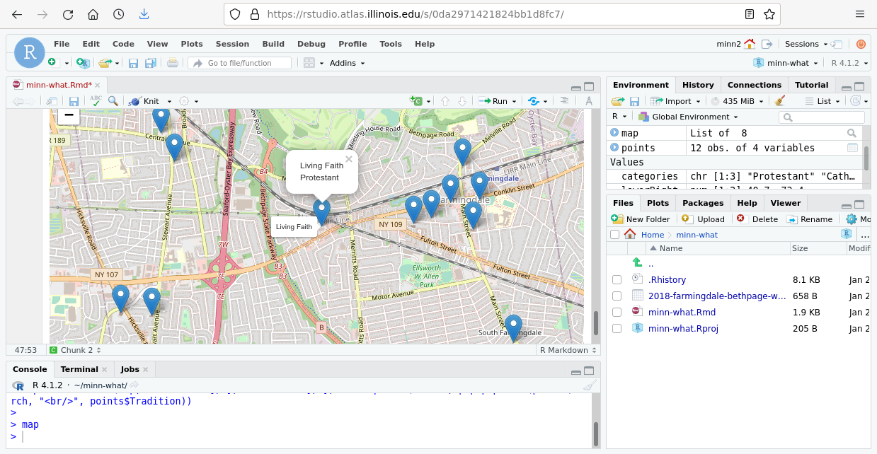
map