Geospatial Data
Revised 14 February 2026
Geospatial data indicates what is where. One of the special things about geospatial data is that it comes in those two parts: what and where.
Attribute (what) data and location (where) data are fundamentally different things and have different characteristics.
A distinction can be drawn between data, information and knowledge with data being raw facts or numbers and information being the interpretation of data that forms the basis of knowledge. However, the three terms are often used interchangeably and interpreted differently by different people, so you should use caution and consider context when you hear or use these words.
Location Data
Latitude and Longitude
The Earth is a spheroid - it is round like a ball or sphere but flattened by slightly by the centrifugal force of rotation. The Earth is 24,900 miles circumference, but around 27 miles wider than it is tall.
To specify locations on the surface of the earth, we use angles that describe where those locations are relative to the center of the earth. Angles across the surface of the earth are measured in degrees, which are subdivisions of circles where one degree represents 1/360th of a circle.
While we think of and experience distances on the planet in terms of length (feet, miles, kilometers) rather than angles (degrees), the earth is lumpy and it is difficult to reliably and consistently measure distance and location across undulating terrain. Even if the Earth's surface were perfectly smooth, manipulating distances across a three-dimensional surface requires fiendishly complex calculations, so specifying locations in degrees is simpler and more accurate than specifying locations in distances.
Since the earth is a three-dimensional object, two angles are required to specify locations on the surface of the earth.
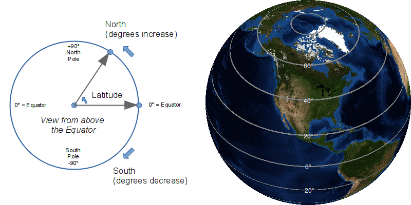
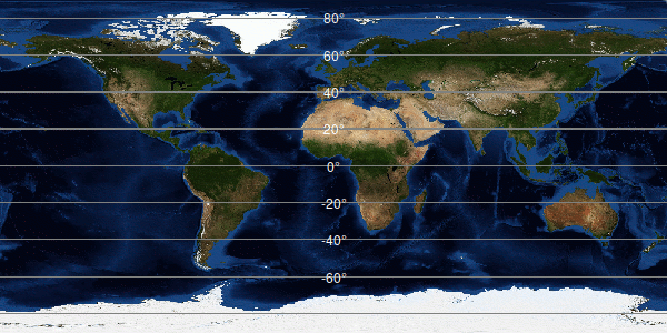
Latitude is the angle that tells you how far you are north or south of the equator. The equator is zero degrees latitude and, commonly, negative numbers are south, positive numbers are north. The range is from negative 90 degrees at the South Pole to positive 90 degrees at the North Pole. Lines on maps are drawn east/west around the planet to show latitude.
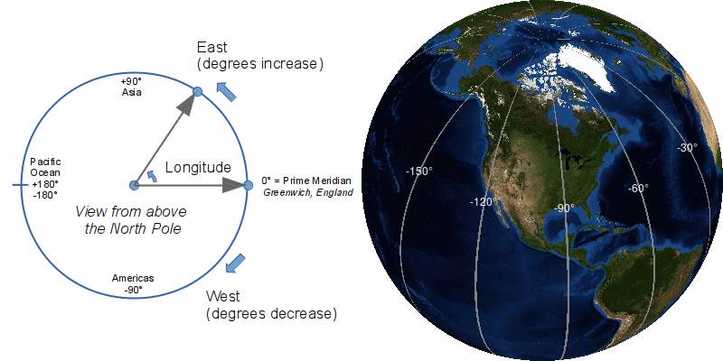
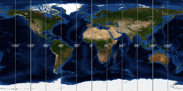
Longitude is the angle that tells you how far you are east or west from the prime meridian in Greenwich, England (longitude 0.0). Think LONG (itude) stretching across your body. Negative numbers up to negative 180 are west of England and positive numbers up to positive 180 are east of England. Lines on maps are drawn north/south between the poles to show longitude.
The Prime Meridian and the International Date Line
Latitude is based on specific physical characteristics of the earth. Zero degrees is set at the equator, the imaginary line around the center of the spinning earth. The axis of the Earth's rotation also happens to point at Polaris (the North Star), a very bright star in the northern sky. It is possible to find your latitude in the northern hemisphere by measuring the angle of Polaris above the horizon using a device like a sextant or astrolabe.
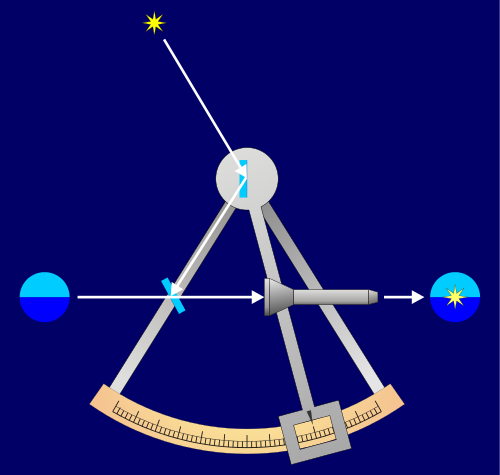
Longitude is more difficult to find than latitude since there are no clear geological or celestial features to define where zero degrees longitude should be located.
Early naval navigators had to carry clocks on their ships to keep track of the time at a location of known longitude. When the sun was directly overhead (12:00 noon), the navigators could tell how many degrees east or west they were of that known longitude by multiplying the number of hours difference between their local 12:00 noon and the 12:00 noon at that known location by 15 degrees (360 degrees rotation of the planet divided by 24 hours in one rotation). Longitude has an interesting history.
The prime meridian is a north-south line that specifies where longitude zero degrees is located. Greenwich, England was chosen as the prime meridian by agreement at a conference of 25 nations called by US president Chester Arthur in Washington, DC in 1884. This was a time when Britain was at the height of its imperial and maritime dominance and this conference simply formalized what was already a common practice on printed nautical charts. The United States government had already started mandating use of the Greenwich meridian in 1850 for nautical purposes.

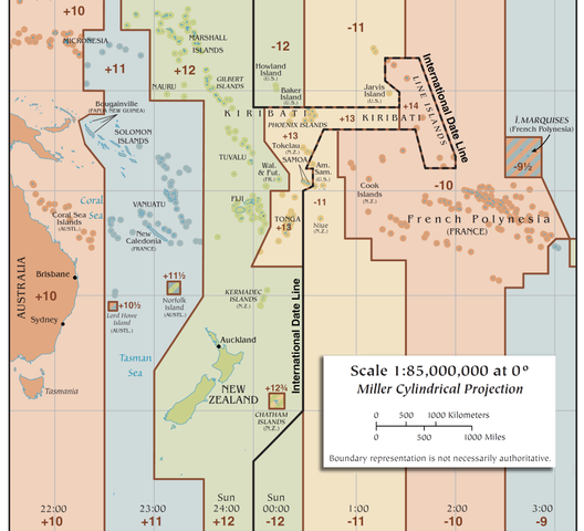
On the opposite side of the planet is the International Date Line. Unlike the prime meridian, this line is not exactly -180 (or +180) degrees longitude, but weaves its way around different islands to deal with political and economic considerations.
Coordinates
A specific location on the surface can be specified with a longitude and a latitude. This pair of numbers is called a set of coordinates. The challenge with geographic coordinates is that there are multiple ways of expressing them.
The traditional form of coordinates is degrees, minutes, seconds (DMS), with a minute being 1/60th of a degree, a second being 1/60th of a minute, North (N) or South (S) meaning north or south of the equator, and East (E) or West (W) means east or west of the prime meridian.
38° 53' 50" N, 77° 02' 12" W
The traditional degrees-minutes-seconds method of specifying coordinates is clear and easy to read by humans, but that type of notation is cumbersome for computers to work with and may not be understood by all GIS software.
With geospatial technology, coordinates are generally specified as decimal coordinates, with positive latitudes meaning north of the equator and negative longitudes being west of the prime meridian.
Decimal coordinates contain only numbers, decimal points, signs, and (sometimes) a comma separator.
38.897192, -77.03896
An additional challenge with decimal coordinates is that although latitude is usually given as the first number (lat-long), sometimes longitude is the first number (long-lat), which is consistent with the convention in geometry where coordinates on a two-dimensional grid are specified as X,Y. If you are plotting coordinates and your points are appearing in unexpected places, this may be due to reversed lat/long.
For example, the WKT (well-known text) representation of a point places the x (longitude) value first:
POINT(-77.03896 38.897192)
With GIS software, it is generally best to stick with latitude, longitude order. You can verify that your coordinates are lat/long by typing them into the search bar in Google Maps.

(The White House 2016)
Elevation
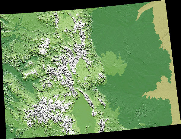
In many situations it is adequate to reference locations with two dimensions (X and Y, or longitude and latitude) since maps and computer displays are in two dimensions. However, we live in a three-dimensional world. Elevation (altitude or Z) is sometimes given as a third coordinate.
Unlike latitude and longitude which are angles given in degrees, elevations represent linear distance above the surface of the earth in feet or meters. While elevation is often specified as height above mean sea level, different applications use different reference points. GPS uses height above the reference ellipsoid (see below).
Geospatial data that includes elevation is usually called 2.5-dimensional (2.5-D) rather than 3-dimensional (3-D) because for each X/Y (longitude/latitude) coordinate there is only one Z (elevation) value. 2.5-D data cannot fully represent structures like buildings that have multiple levels or floors stacked on top of each other at different elevations for each X/Y coordinate.
Datums
Reality rarely quantifies exactly to simple mathematical models, so the topic of elevation also raises an issue with exactly how the pure, spherical angles of latitude and longitude reflect the rugged, three-dimensional reality of the earth. In addition to the planet being slightly flattened from a perfect sphere by the force of rotation, the surface is covered with lumpy mountains and oceans. If you want to be very precise about locations (such as when engineering a bridge or dropping a bomb on someone) these lumps can result in errors that can cause problems.
This challenge is addressed in cartography in three stages:
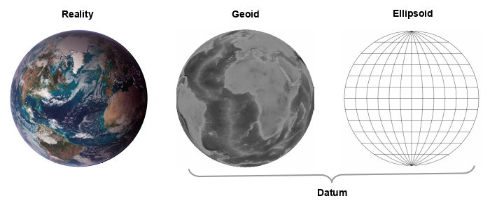
- A geoid is an estimate of the lumpy shape of the earth.
- A reference ellipsoid is a perfectly smooth mathematical estimate of the geoid.
- A geodetic datum is a coordinate system and set of reference points drawn across the ellipsoid. A datum always specifies both a geoid and an associated ellipsoid.
- That datum is then used to convert latitude, longitude, and elevation to specific locations on the surface of the earth with high accuracy.
There are a number of different datums that are used in different parts of the world, for different purposes, and at different times. These different datums reflect:
- Fitting to specific parts of the earth
- Improvements in measurement technology
- Changes in the earth's topography, such as the shifting of tectonic plates
Datums you will commonly encounter in the US include:
- World Geodetic System of 1984 (WGS 84): The datum used by GPS
- North American Datum of 1983 (NAD 83): A datum specifically tailored to closely fit North America
- North American Datum of 1927 (NAD 27): An obsolete datum you will find used on older maps

Data Models and Geometry
There are two broad models for storing geospatial data: vector and raster. Of the other types of models, point clouds are increasingly being used in GIS. They are called models because they are simplified representations of the objects or phenomena they are used to represent.
Vector Data
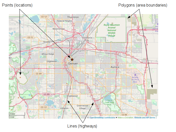
Vector data stores locations as discrete geometric objects: points, lines, or polygons.
- Points are represented with a single coordinate pair (latitude and longitude). Points useful for representing objects like vehicles or smartphone locations that occupy little or no area
- Polygons are represented with a collection of coordinate pairs that define the outside boundary of an area. Polygons are useful for representing things like property boundaries or city boundaries that define an area
- Lines are represented by a sequence of coordinate pairs. Lines are useful for representing things like roads or paths that are long and narrow
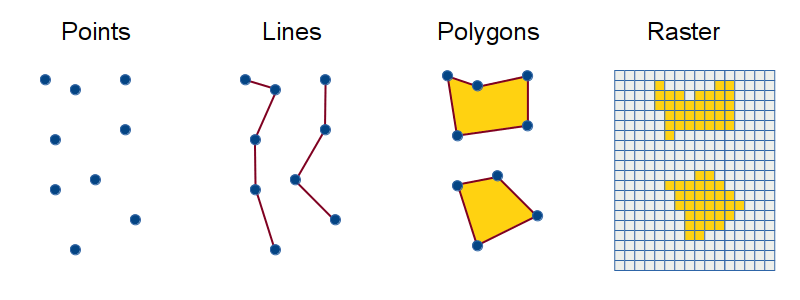
Areas are occasionally represented with centroids, which are points in that are mathematically equidistant from all parts of the area. For example, the political boundaries of cities are best represented with an area, but on a large map covering an entire nation, individual cities may be represented with points to make the map easier to read.
Raster Data
Raster data is stored in a grid of regularly-spaced pixels of attribute data that cover an area of interest. Raster data is most useful for representing data about areas where there are unclear boundaries, such as with elevation, temperature or amounts of vegetation. The best known type of data is photographic image data. The digital elevation model described above is another example of geospatial data stored in rasters.
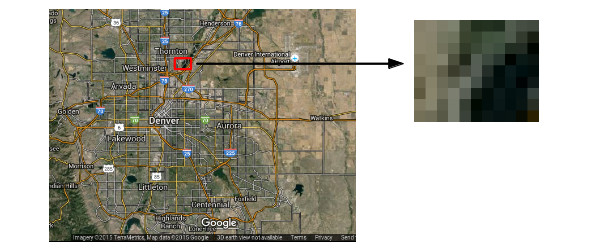
Although many different types of data can be stored as rasters, data about discrete objects with clear boundaries is usually more appropriately and accurately stored as vector rather than raster. GIS Software allows conversion between raster and vector, although the conversion process between the two models often involves inaccuracy and uncertainty.
Point Clouds
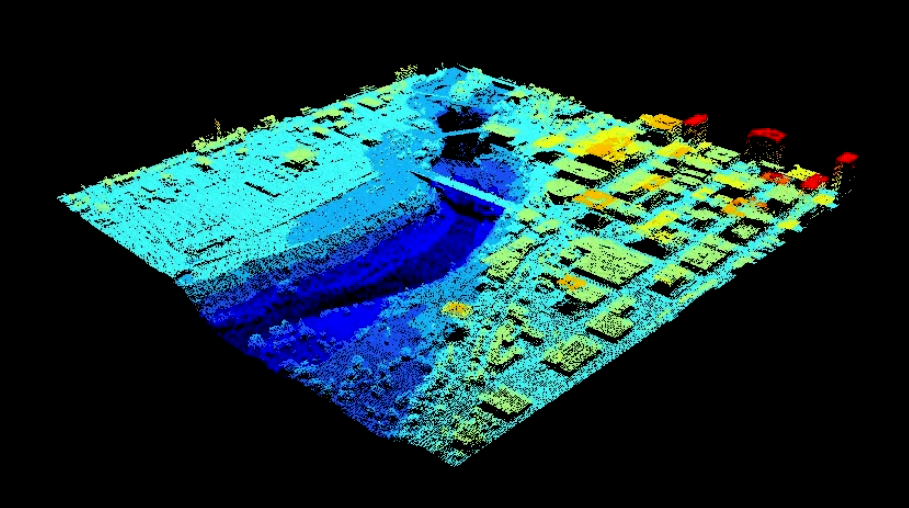
An emerging third type of model is the point cloud, which stores geospatial information as a collection of points in three-dimensional space (latitude, longitude and elevation). Point clouds are commonly captured using a aerial laser scanning technique called lidar. Unlike vector and raster data that is analogous to a flat two-dimensional map, point clouds can be used to more-faithfully represent structures and topography, albeit at the cost of greater storage and processing demands.
Attributes
Spatial locations by themselves generally aren't particularly useful and you need some what to go with the where.
Attributes are text or numbers that represent the what part of what is where in geospatial data.
Attributes are also sometimes referred to as fields, variables, or columns.
Variable Types
Variables can be classified by the types of information they represent. The classification is important because it determines what kind of analysis can be performed on that attribute, and what kinds of charts or maps are appropriate for visualizing that attribute.
The classification scheme derived below is an elaboration of the levels of measurement commonly used in statistics (Stevens 1946).
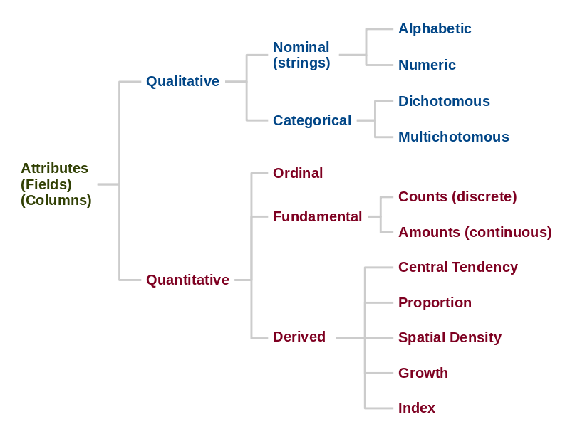
- Qualitative variables represent qualities of places, people, or things that are too subjective, ambiguous or irregular to be easily converted to simple numbers.
- Nominal variables are names or descriptions or individual things, usually represented in storage as character strings.
- Alphabetic data consists of text. Examples:
- Names of US state capitals in 1865
- Names of art museums in Chicago in the 1990s
- Personal names of homeowners in Yankee Ridge in 2022
- Descriptions of top California wineries in 2021
- Numeric nominal data is composed of digits, but unlike quantitative data, you cannot meaningfully perform numeric operations like adding or averaging on these numbers. Examples:
- Athletic jersey numbers of Chicago Bulls players in 1977
- Social Security numbers of participants in a 2022 vaccine trial
- Categorical variables are names used to divide individual things into groups. Categorical data is often considered a specific type of nominal data.
- Dichotomous variables represent categories with only two possible values. Examples:
- Whether individual families in Danville have children in 2023 (yes / no)
- Wildfire risk in different state parks in Illinois in the summer of 2020 (High / Low)
- Multichotomous variables represent categories with more than two possible values. Examples:
- Political affiliation of individual residents of a city in November 2022 (Democratic, Republican, Green, Independent, etc.)
- Religion associated with specific houses of worship in Springfield in 2022 (Muslim, Catholic, Protestant, Buddhist, etc.)
- Quantitative variables represent characteristics as quantities or numeric values.
- Ordinal variables rank items in order. Examples:
- Individual voter approval of a mayoral candidate in October 2022 on a scale of 1 (lowest) to 5 (highest) (Likert scale)
- Rankings of individual basketball teams in the Big-10 at the end of the 2022 season
- Fundamental variables are numbers that represent empirically observable characteristics (Stevens 1946).
- Counts are numeric characteristics that can be counted with
no fractional parts. Counts are also referred to as whole numbers or
discrete data. Often represented in storage as integers, although
real numbers can be used when the possible values exceed
the maximum value that can be represented with an integer. Examples:
- Population of countries in 2019 (there are no half people)
- Number of votes for Joe Biden by county in 2020
- Number of sunny days by major city in the US in 2020
- Amounts are numeric characteristics that are measured. These
characteristics do not necessarily fall exactly on integer boundaries
and are represented with numbers that have decimal points. Also
referred to as continuous data. Represented in storage
with real numbers. Examples:
- Annual household income for individual residents in Springfield in 2022
- Gross domestic product by country in 2015
- Maximum summer temperature in Illinois cities in 2022
- Derived variables are numbers that are calculated by performing mathematical operations on fundamental values.
- Proportions are the fraction that something is of a whole. Examples:
- Percent of population that is obese in each state in 2022
- Number of violent crimes per 10,000 residents in 2022
- Central tendency is a single central (middle) value used to summarize a set of numbers. Examples: mean (average), median, mode, per-capita. Examples:
- Median monthly housing cost by state in 2017
- Per-capita gross domestic product (GDP) by country in 2020
- Mean annual PM 2.5 exposure by country in mg per cubic meter in 2019
- Growth is a percentage change from a prior time. Examples:
- Indices are values representing different characteristics that are combined into a single number. Examples:
- Spatial density is the amount of something within a particular unit of area. Examples:
- Residents per square mile in each US zip code in 2018
- Bushels of corn harvested per acre of farmland in Champaign County in 2002
Variable Aspects
Geospatial variables have different aspects that work together to represent objects or characteristics on the surface of the earth.
Quantitative variables always have a unit, which is a name that indicates what the numbers represent.
A number without a unit is meaningless. For example, the number 70,000 means nothing by itself, but $70,000 in household income makes that number useful.
Quantitative and qualitative variables have some or all of the following aspects:
- Characteristic: What is the phenomena being named, categorized, counted, or measured? Examples:
- Residents
- Household income
- Air temperature
- Body weight
- Time period: What range of time is covered by each value? Examples:
- In 2022 (year)
- In the 1990s (year range)
- On January 6, 2021 (specific date)
- At 12:00 pm on January 20, 2021 (specific time)
- Area type: What location or area is being covered by each of the values? Examples:
- By country
- By state
- By person
- By facility
- Measurement unit: What unit is used as the standard for specifying quantitative values? Examples:
- Degrees
- Kilograms
- Dollars
- Number of (population)
- Aggregation: How are multiple values in an area aggregated to a single variable value? Examples:
- Total (Sum)
- Mean (Average)
- Median
- Rate: How does the variable quantify difference or change over time and space? Example:
- Percent
- Per capita
- Per square mile
- Per hour
- Multiplier: How is the variable value transformed to make it more readable? Example:
- Thousands
- Millions
- x*10y (scientific notation)
Variable Descriptors
A descriptor is "a word or phrase (such as an index term) used to identify an item (such as a subject or document) in an information retrieval system" (Merriam-Webster 2023).
For the purposes of this tutorial, a variable descriptor is a short phrase that describes the different aspects of a variable so the user can understand exactly what the variable values represent.
- Average sales in dollars by store in April 2020
- Aggregation: average
- Characteristic: sales
- Measurement: in dollars
- Area type: by store
- Time period: April 2020
- Total population in Illinois counties in 1890
- Aggregation: total
- Characteristic: population (residents)
- Area type: in Illinois counties
- Time period: 1890
- Stroke mortality per 100K residents by state in the year 2016
- Characteristic: stroke mortality (deaths from stroke)
- Rate: per 100K residents (100,000)
- Area type: by state
- Time period: in the year 2016
- State renewable energy portfolios in 2022
- Area type: state
- Characteristic: renewable energy portfolios (mandatory, voluntary, none)
- Time period: in 2022
Data Considerations
Geospatial vs. Non-Geospatial Data
Geospatial data is distinguished by having multiple where, while non-geospatial data has one where or no where.
Because space and time are tied together, geospatial data also has a when (temporal dimension).
| Geospatial (multiple where) | Non-Geospatial (zero or one where) |
|---|---|
| Names of the different birthplaces of 2022 Chicago Cubs players | Names of 2022 Chicago Cubs players |
| Number of Chinese restaurants by US metropolitan area in 2022 | Number of Chinese restaurants in Chicago in 2022 |
| Annual rainfall at each airport in Illinois in 2022 | Annual rainfall for each year between 1972 and 2022 at Chicago O'Hare airport |
| Median household income by state in 2022 | Median household income in Illinois in 2022 |
Accuracy vs Precision
The precision with which you express a number should be in keeping with the amount of accuracy that your data possesses.
- Accuracy is how close your count or measurement reflects the reality that you are counting or measuring.
- Precision is the amount of accuracy that you express with the numbers you use to represent your data. Usually what this means is the number of significant digits used. For example:
- 1.2345123 is more precise than 1.2
- 45,000,000 is less precise than 45,244,391.224
Example:
- The measured temperature on three days was 73, 76 and 78 degrees (two significant digits of precision)
- A calculator might calculate and display the average (mean) temperature as 75.666666667
- Since you have only two significant digits in your source data, you do not have 11 digits of accuracy implied by the 11 digits of precision
- Rounding and writing the mean as 76 degrees or 76 2/3 degrees would keep the precision and accuracy in harmony
Precision is often used to deceive people into thinking that you have a better understanding of reality than you actually do. For example:
- You say that 12,456 people attended your campaign rally
- The assumption from that statement is that you have an accurate account of attendance and that you are a confident, well-informed candidate worthy of election
- However, that number is just describing a rough estimate between 5,000 and 15,000 since people come and go from campaign rallies and often are not being accurately counted when they enter or leave an area
- Your highly precise statement is deceptive because you don't really have a count as accurate as the precision of your statement implies
Spatial Accuracy vs Precision
The world is thing of infinite, wondrous complexity.
When we try to understand that world as numbers, we have to simplify. Our measuring devices and techniques cannot be exactly accurate. We have to round numbers so our precision reflects our accuracy.
With latitudes and longitudes in degrees, the number of decimal places you use (precision) reflects the accuracy of that location on the ground. That accuracy can be expressed as +/- a distance on the ground.
The table below shows the approximate distances for each fraction of a degree in Manhattan:
| Degrees | Latitude | Longitude |
|---|---|---|
| 0.1 | 6.91 miles | 5.23 miles |
| 0.01 | 3,648 feet | 2,764 feet |
| 0.001 | 365 feet | 276.4 feet |
| 0.0001 | 36.5 feet | 27.6 feet |
| 0.00001 | 43.8 inches | 33.2 inches |
| 0.000001 | 4.38 inches | 3.32 inches |
| 0.0000001 | 11.1 millimeters | 7.02 millimeters |
| 0.00000001 | 1.11 millimeters | 0.702 millimeters |
Primary vs Secondary Data
Primary data is data you capture yourself.
Secondary data is data you recycle from someone else.
Primary data is often more expensive to obtain since you will have to do work to get it, such as by surveying with GPS devices or conducting surveys with human subjects. But if you're doing something novel, you will likely need novel data that you get yourself rather than from someone else.
Population vs Sampled Data
Generally, the more data you have, the better your conclusions when you analyze that data. If you have population data for everything you are studying, that is ideal.
An example of population data is the census conducted every ten years, where the US Federal Government attempts to find and count every person in the country and get basic information on who they are and where they live (what is where).
However, in many if not most research situations, it is too difficult or expensive to capture complete data. For example, if you are running a congressional campaign, you cannot survey every voter in your congressional district to find out how they are planning to vote.
In such cases it is usually adequate to capture a sample of the data and then use statistical techniques to make an inference from that sample about the full population. The use of sampling rather than a full census introduces uncertainty about whether your sample reflects the overall population.
However, there is always some uncertainty when gathering data (especially about humans) and the uncertainty with sampled data can be quantified and considered as part of the analytical process. The uncertainty associated with sampled data is expressed as a margin of error, which is a range of values above and below the estimated values. Margins of error are typically given that specify a 95% confidence interval, which means that we can be 95% certain that the actual value falls within the margin of error above and below the value estimated from the sample.
Individual vs Aggregated Data
Individual data is data about individual persons or objects.
Aggregated data is data that combines data from groups of individuals (often based on location in different geographic areas) into a smaller set of numbers, usually averages or medians. An example of aggregated data is US census data that is aggregated by census tract or county in order to preserve the privacy of individual census respondents.
As with sampling, aggregation introduces uncertainty as important individual distinctions can be lost when people are combined into groups and summarized.
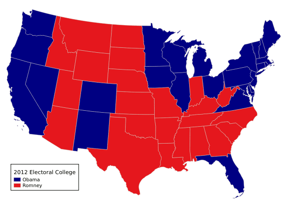
One issue with aggregated data is the ecological fallacy, when you make assumptions about individuals based on aggregated data. For example, states are often classified as red states or blue states based on whether the majority of the voters in that state vote Republican or Democratic, respectively. However, even in very red Utah, Democratic President Obama got 25% of the vote in the 2012, so assuming that everyone you meet in Utah is conservative is incorrect.
The opposite of the ecological fallacy is the
exception fallacy, where an assumption is made about
a group based on a few exceptional individuals.
For example, if you meet a tall basketball player from
Ohio, the assumption that everyone in Ohio is tall
would be incorrect.

Structured vs Unstructured Data
Structured data is strictly organized so that for every field or record in your data, you know what it represents. If your data is organized in a table with columns and rows, it is probably structured. Most geospatial data that you deal with in conventional geographic information systems is structured.
Unstructured data is data that is not clearly organized in a way that it can be simply processed by computers. Examples of unstructured data is text like Facebook posts, text messages or tweets. There is meaningful data there, but turning it into something useful requires analysis (often by humans or complex computer algorithms) to give it some kind of structure. Contemporary societies generate tremendous amounts of unstructured data and the analysis and use of that data is an area of heavy research (and investment) called big data.
Metadata
If you don't know what you have, then you don't have it.
Metadata is data about your data. Typical items kept in metadata include:
- Name of the data set
- Overall description of what the data set contains
- Dates of capture, processing, analysis, and/or backup
- Information about the variables (names, ranges, units, etc)
- Information about the location data
- Notes or caveats about the quality and accuracy of the data
- Source and contact information for the people who collected the data
Students often confuse data with metadata. The following table contrasts data with metadata that could be associated with that data:
| Data | Metadata |
|---|---|
| Patient names and addresses | The name of the computer disk file where current patient information is kept |
| Names of participants in a drug trial | The names of the technicians who recorded the drug trial results |
| Test scores | The range of dates when the test scores were captured |
| Hourly temperatures | The location of the sensor where those temperatures were recorded |
| Incidence rates for diseases by state | The names of the agencies that collected the disease data |
While simply remembering what you have is adequate for small projects with short-term needs (like class projects), failure to document your data may make the data useless if you ever want to reuse that data in the future.
- Metadata helps keeping track of your inventory of data when you have a number of different data sets
- Metadata aids in sharing data by making it possible for other people to know exactly what is in your data set
- Metadata can be used as a reminder if you need to use your data in the future and have forgotten details about what the variables mean or where you got the data
- If you are collecting data for published research, you need to be able to provide details about your data so the quality of the research based on that data can be judged.
However, because the creation of metadata is usually separate from the capture and processing of the data itself, and is more about the future than getting the task at hand done, it is common for metadata to be missing or skeletal. While it is often possible to look at the data and make a reasonable guess as to what it represents and where it came from, a few minutes adding metadata can save a great deal of effort in the future for you and for other people who use your data.
Philosophical Considerations

X/Y coordinates are called Cartesian Coordinates after the French philosopher Rene Descartes (1596 - 1650). Descartes is also remembered for is statement Cogito ergo sum (I think therefore I am) as evidence of our own existence.
Cartesian coordinates combines the principles of geometry codified by the Greek philosopher Euclid (c. 300 BC) with the techniques of algebra codified by the Arab mathemetician Muḥammad ibn Mūsā al-Khwārizmī (c. 780–850) to create a useful and powerful synthesis that is a foundation for contemporary geospatial technology.
Descartes coordinate system was part of a broader philosophical quest to find objective knowledge about the world that is independent of our perspective and preconceptions. Descartes believed that the only essential properties of matter were geometric, so an objective understanding of the world could be had through a sufficiently advanced geometry (Shand 2002, pp 72).
Descartes philosophy, to some extent, is a foundation for the geospatial technology that is based on Decartes way of representing the world in his coordinate system. This is also the foundation of a critique of geospatial technology that reducing the world to X/Y coordinates obscures not only important qualitative and subjective meanings, but also obscures the political and economic forces (and associated moral questions) underlying the development and use of geospatial technology.
Geospatial technologies with their vivid visualizations and massive scope, are charismatic, and charisma can deceive.