Visualizing Landsat Data in ArcGIS Pro
Rev. 5 November 2024
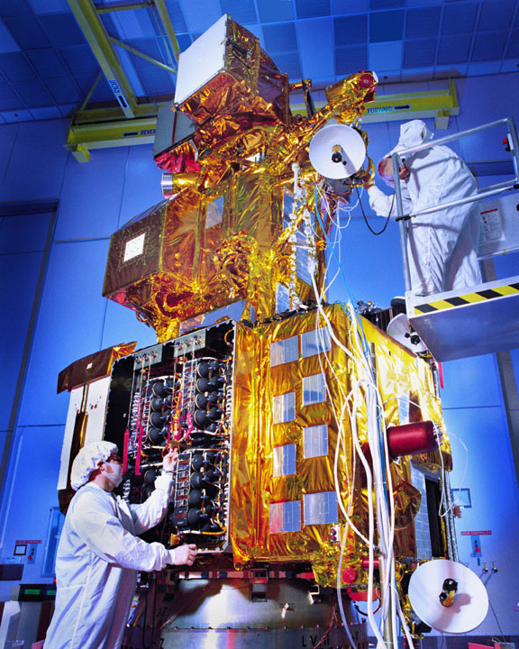
Of the hundreds of remote sensing satellites launched in the past half century, the Landsat program has proved especially valuable for civilian use.
Landsat 1 was launched on 23 July 1972 and subsequent satellites have provided continuous satellite imagery of the Earth. This is arguably one of the most important scientific enterprises of our time, and if you work with remote sensing, you will probably use Landsat data on multiple occasions.
Landsat 8 (launched 11 February 2013) and Landsat 9 (launched 27 September 2021) are currently operational (NASA 2022).
This tutorial will cover the basic visualization of Landsat data in ArcGIS Pro.
Remote Sensing
Remote sensing is "the process of detecting and monitoring the physical characteristics of an area by measuring its reflected and emitted radiation at a distance from the targeted area" (USGS 2019).
While remote sensing is commonly used as a synonym for satellite data, the concept of remote sensing can also be applied to aerial photography or lidar from drones. The remote part of remote sensing means that you are gathering data from a distance.
Raster Data
Satellites almost always capture data as raster data.
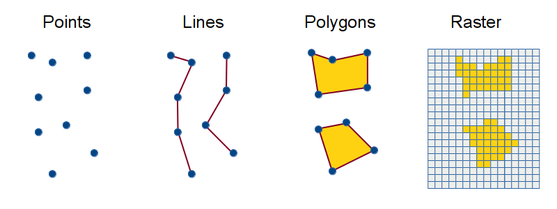
Raster data represent characteristics of areas on the earth
as regular grids of rectangular pixels.
![]()
Raster data is often contrasted in GIS with vector data. Vector data stores locations as discrete geometric objects: points, lines or polygons.
Geographic phenomena can usually be represented using either vectors or rasters, but some types of phenomena are better suited to one or the other.
- Vector data is generally more useful for representing human creations that have clear boundaries, like built structures or political boundaries.
- Raster data is generally more useful for environmental characteristics that do not have clear or stable boundaries, like elevation or vegetation types.
Temporal Resolution
The temporal resolution of available satellite data is how frequently data is available for any particular location on the surface of the earth. Some satellite systems return to the same location daily, while others that are designed to observe the entire earth may take days or weeks to return to the same location.
Each Landsat satellite covers the entire earth every 16 days, and since the two satellites (Landsat 8 and 9) are eight days out of phase, this gives Landsat data a temporal resolution of eight days. Each Landsat satellites completes just over 14 orbits a day in a near-polar, sun-synchronous orbit so they spend as much time as possible looking at areas of the earth lit by the sun.
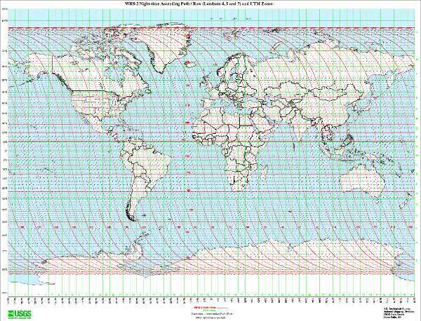
Landsat data is publicly available as scenes (images) that cover an area around 100 miles square. Scenes are designated by a path number (scanning path west to east) and row number (scene location on the path south to north).
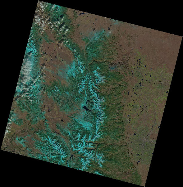
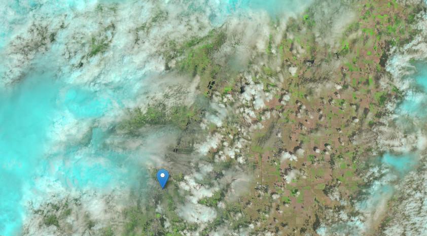
The scene below was acquired from Landsat 8 on 10 November 2015. It is path 34, row 32, covering North Central Colorado with Denver in the lower right-hand corner.
While temporal resolution of captured data is determined by the orbit, the temporal resolution of usable data can be affected by cloud cover. If an area is obscured by clouds when the satellite passes over, that data may be unusable and no data can be captured for that area until the satellite passes again when there are fewer clouds. This can be a significant problem when attempting to use Landsat data for areas that have cloudy climates where long successions of scenes may be partially or totally obscured.
Spectral Resolution
Remote sensing takes advantage of the emission and reflection of electromagnetic radiation by objects on the surface of the earth to capture what is where on the surface of the earth.
The spectral resolution of a remote sensing system is the range of electromagnetic radiation frequencies captured by the sensor. Satellite sensors capture ranges of frequencies in bands and the spectral resolution of a satellite sensor is usually specified by the numbers of different bands available and the ranges of frequencies covered by each band. The appropriate spectral resolution depends on the purpose of the satellite.
Landsat 8 and 9 capture data in 11 different bands, giving Landsat 8 and 9 a spectral resolution that includes visible light, near-infrared, short wave infrared, and thermal infrared bands (USGS 2017).
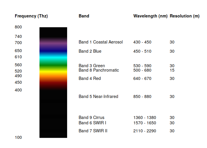
The diagram below shows the relationship of Landsat bands 1 - 9 to the visible light spectrum. Bands 10 and 11 captured by the Thermal Infrared Sensor (TIRS) are much lower frequencies and are not shown.
Spatial Resolution
Spatial resolution represents the amount of area on the surface of the earth covered by each pixel. Spatial resolution is usually measured by the distance in meters between the centers of adjacent pixels.The level of spatial resolution determines the level of detail that can be distinguished in a remotely sensed image. As you zoom in closer to the earth, the amount of information available diminishes and the images appear more fuzzy.
Landsat 8 and 9 spatial resolution is 30 meters for most bands, except for 15 meter resolution with panchromatic (grayscale) band 8 and 100 meter resolution with thermal infrared sensor bands 10 and 11 (USGS 2017).
Landsat data is available in three different levels (USGS 2020).
- Level 1 data has undergone a basic level of processing (radiometric calibration and orthorectification) so that it can be used for basic visualization and analysis.
- Level 2 data is level 1 data that has been corrected for the effects of water in the atmosphere so that areas can be compared across scenes captured at different times.
- Level 3 data has additional specialized processing to analyze surface water, snow cover, and areas that have been burned in wildfires.
Downloading Landsat Data
The USGS makes recent and historic Landsat data freely available via the EarthExplorer website.
In order to download data, you need to register (for free). Click the Login button and select Create New Account.
Once you have registered, you can log in and download scenes.
- Log in.
- Search for a location that you want to explore (Champaign, IL).
- For the data set, use:
- Landsat
- Landdsat Collection 2 Level-1
- Landsat 8/9 OLTI/TIRS C2 L1
- View scene footprints that are in the time frame of interest, that cover your area of interest, and are not covered in clouds. Be aware that for vegetation analysis, summer scenes are better.
- Click Download and you will be given multiple options. Download the Full-Resolution Browse (Reflective Color) GeoTIFF.
- Select Product Options for the Landsat Collection 2 Level-1 Product Bundle and download the following:
- xxx_B2.TIF (blue)
- xxx_B3.TIF (green)
- xxx_B4.TIF (red)
- xxx_B5.TIF (near infrared)
Browse Images
USGS publishes preprocessed color scene images that can be downloaded directly without having to combine band files or perform additional correction.
Landsat Full-Resolution Browse (Reflective Color) GeoTIFF scenes are actually false-color images constructed with SWIR I, near-infrared, and red bands (bands 6, 5, and 4), but they often provide a clearer view of a scene and require much less work to use than images created from the red, green, and blue band files (bands 4, 3, and 2) (USGS 2024).
- Create a new map and give it a meaningful name.
- Add Data with the natural color TIFF file (*_RT_refl.tif).
- Loading may take a few seconds. If asked to Build Pyramids, click OK.
- If you zoom in closely you can see the individual square pixels. To smooth out the edges, in the Raster Layer ribbon, change the Rendering and Resampling Type to Bilinear or Cubic.
- Also in the Raster Layer ribbon, change the Layer Blend to Multiply. This will use the image to color the base map, while keeping the labels and feature outlines from the base map visible.
- Create a layout and export as needed.
Visualizing Composite RGB Images
Composite RGB images combine red, green, and blue bands of visible light to show the scenes more closely to the way they would appear if you were viewing the earth from space. You can use the individual red (band 4), green (band 3), and blue (band 2) files from the Level-1 GeoTIFF Data Product data.
- Create a new map and give it a meaningful name (RGB Map).
- In the Analysis ribbon, click Tools open the Composite Bands tool. This will combine the different file bands into a single layer.
- Add your three color bands as Input Rasters. Add B4 (red), then B3 (green), and finally B2 (blue) in that order so the software knows which band is which.
- Give the Output Raster a meaningful name (RGB_Composite).
- After 30 seconds or so, the composite raster should be added to the map as a color image.
- In the Raster Layer ribbon:
- Change the Layer Blend to Multiply. This will use the image to color the base map, while keeping the labels and feature outlines from the base map visible.
- Under Rendering change the Resampling to Cubic to give clearer rendering when zooming in.
- Under Rendering change Stretch Type to Standard Deviation so the range of displayed levels is more in keeping with common expectations about how terrain should appear.
- Create a map layout and export, if needed.
Normalized Difference Vegetation Index
Bands other than visible light are useful for analyzing a variety of phenomena. For example, biogeographers commonly use a combination of red and near-infrared bands called normalized difference vegetation index (NDVI) to determine levels of vegetation in a particular area.
NDVI is based on a characteristic that photosynthetic green plants tend to reflect infrared light to avoid overheating, but absorb red light to power the process of photosynthesis.
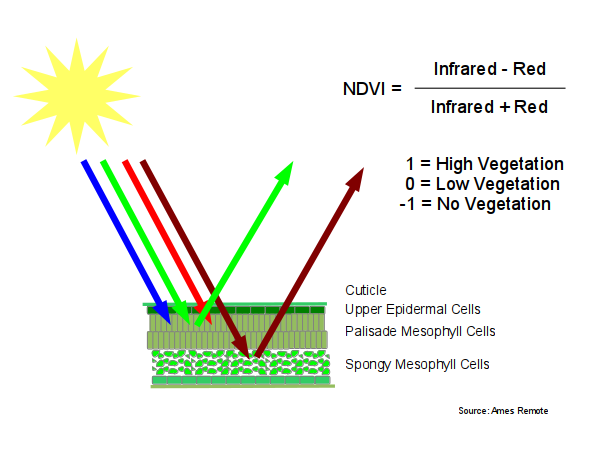
The range of the index is negative one to positive one.
When near infrared is high and red is low, that is when living photosynthetic plants are reflecting infrared and absorbing red, making NDVI high and closer to one.
1 - 0
----- = 1
1 + 0
When near infrared is low and red is high, such as with bare ground or water, NDVI is low and closer to negative one.
0 - 1
----- = -1
0 + 1
The normalization specified in this formula provides NDVI values that are useful regardless of variations in the level of lighting or the angle of view. It also makes it possible to distinguish between photosynthetic vegetation and non-photosynthetic green areas (like artificial turf). Accordingly, this gives NDVI an advantage over simply looking at an RGB image for areas that appear green.
This phenomena can be used with the Landsat 9 near infrared band (band 5) and the red band (band 4) to calculate an index that is highest in areas with large amounts of vegetation, and lower in areas of low vegetation.
Because NDVI creates a set of values from -1 to +1 and has no color of its own, maps of NDVI are commonly visualized with false-color that assigns different colors to ranges of values and makes areas with high and low NDVI easier to distinguish.
- Create a new map and give it a meaningful name (NDVI Map).
- Add Data with the red band (B4) and near-infrared band (B5) GeoTIFF files.
- Rename the layers to their colors so the names are more meaningful (B4 = Red, B5 = Infrared).
- In the View ribbon, click Geoprocessing open the Raster Calculator tool. This will allow you to calculate an NDVI layer from the red and near-infrared bands.
- In the Map Algebra Expression box, enter the formula for NDVI using
the raster layer names:
("Infrared" - "Red") / ("Infrared" + "Red") - Give the Output raster a meaningful name (NDVI).
- The layer will automatically be added to the map as a grayscale layer with lighter colors of higher NDVI values (more vegetation) and darker colors of lower NDVI values (less vegetation).
- Change the Symbology to false color so the areas of vegetation stand out more clearly.
- In the Raster Layer ribbon, change the Layer Blend to Multiply and the Resampling to Cubic.
- Hide the individual band layers.
- Create a map layout (NDVI Layout) and add the map frame.
- Add a legend.
- Add annotations if desired.
Save Your Project
You can save your project as a Project Package to ArcGIS Online in case you need it in the future.
Note that Landsat raster scenes are quite large, so saving the package may take a few minutes.
If you get a message, "There is not enough space in your online account to upload the package," try selecting the "Save package to a file" option and then going into your ArcGIS Online Content web page and uploading that .ppkx file.