Brownfields Analysis in R

All spaces go through a life cycle, and industrial sites are often abandoned as a result of changes in technology, economics, or politics. These abandoned sites often have water and soil contamination that can effect the health of local communities long after the industrial activities at those sites have ceased.

Brownfields are "abandoned or under-used industrial and commercial properties with actual or perceived contamination and an active potential for redevelopment" (Illinois Environmental Protection Agency 2021).

Superfund sites are abandoned industrial sites that have been designated by the US EPA to be part of a program created by the Comprehensive Environmental Response, Compensation, and Liability Act. CERCLA was passed in 1980 to provide federal funding to clean up uncontrolled or abandoned hazardous-waste sites as well as accidents, spills, and other emergency releases of pollutants and contaminants into the environment. This program is commonly referred to as the Superfund.

EPA uses a variety of legal techniques to get private potentially responsible parties to clean up these sites. EPA cleans up these sites on its own when responsible parties cannot be cannot be identified or located, or when they fail to act (EPA 2020).

This tutorial will cover analysis of Superfund sites in R.

Acquire the Data

Cleanup Sites

Industrial cleanup sites targeted by the EPA are published on the EPA's Cleanups in My Community site, although the process is cumbersome and the downloaded files need processing to be suitable for spatial analysis.

Go to the Cleanups in My Community main page.
Scroll to the middle of the page and select "Create a listing of cleanup sites or grants..."
Select the area you want. For this example we choose State/Territory and Illinois.
Select only the Superfund NPL sites (national priorities list).
Apply the filter.
Under the Actions selection box, choose Download.
For Choose report download format, select CSV.

Downloading Illinois Superfund site information from the EPA

Cancer, Demographic, and Toxics Releases Data

Cancer data for this tutorial was originally sourced from the Illinois State Cancer Registry.

Demographic data for this tutorial was originally sourced from the American Community Survey 2015-2019 five-year estimates.

Toxics releases data was originally sourced from the the EPA Toxics Releases Inventory program page.

Download and processing of this data is described in the tutorial Toxics Releases Analysis in R.

You can download a GeoJSON files of the toxics releases facilities here and the cancer and demographic data by ZIP Code here.

Map of estimated pounds of industrial carcinogen releases by ZIP Code in Illinois in 2019

Process the Data

Load a Base Map

Because many of the features analyzed in this tutorial are isolated points or areas, it will often be helpful to plot() those points over a base map.

The OpenStreetMap library provides functions for accessing base map tiles from OpenStreetMap (OSM), which is a common open source geographic information source. OpenStreetMap is like Wikipedia for geospatial data.

Sys.setenv(NOAWT=1)

library(OpenStreetMap)

basemap = openmap(upperLeft = c(43, -95.5), lowerRight = c(37, -83.5), zoom=6)

plot(basemap)

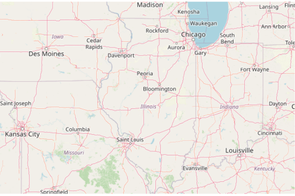
The Sys.setenv(NOAWT=1) call indicates that the OpenStreetMap package should not use the java.awt classes for creating user interfaces and for painting graphics and images, since a display may not be available if you are using this code on a server. This should address the java.awt.AWTError: Can't connect to X11 window server using ':0' as the value of the DISPLAY variable error.

Load Cleanup Sites

The complete list of cleanup sites can be loaded into a data frame using the read.csv() function.

cimc = read.csv("cimc_basic_search_result.csv", as.is=T)

names(cimc)

	 [1] "Cleanup.Name"         "Location.Address"     "City.Name"           
	 [4] "State.Code"           "Postal.Code"          "County.Name"         
	 [7] "EPA.ID"               "Brownfields.Link.CSV" "RCRA.CSV"            
	[10] "Superfund.Link.CSV"   "ECHO.Link.CSV"        "Response.Link.CSV"   
	[13] "RE.Powering.CSV"      "FRS.Link.CSV"         "Map.Site.CSV"

Sites on this list include:

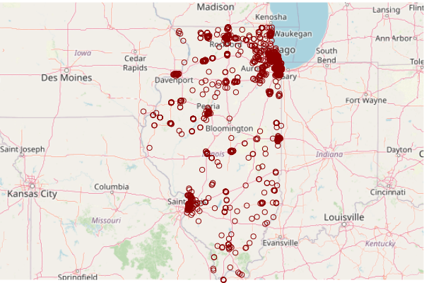
Convert to Features

Although there are no latitude/longitude location fields, the Map.Site.CSV URL to the EPA's mapping site contains latitudes and longitudes in the URL that can be extracted using the sub() function that substitutes (replaces) text based on regular expressions.

latlong = sub(".*GEOSEARCH:", "", cimc$Map.Site.CSV)

cimc$Latitude = as.numeric(sub(" .*", "", latlong))

cimc$Longitude = as.numeric(sub("[0-9\\.]* ", "", latlong))

The latitude and longitude columns can then be used to create features.

st_as_sf() converts the numeric lat/long columns to features.
The base map is plot() first so the points are drawn on top of it.
st_geometry() isolates only the location part of the feature so that plot() does not try to draw separate maps for all of the different attributes.
st_transform() converts the features to the projection of the OSM base map. A projection is the mathematical transformation that converts lat/long angles on the surface of the three-dimensional earth to two-dimensional map.

library(sf)

cimc = cimc[is.finite(cimc$Latitude),]

cimc = st_as_sf(cimc, coords = c("Longitude", "Latitude"), remove=F, crs = 4326)

plot(basemap)

plot(st_transform(st_geometry(cimc), osm()@projargs), col="darkred", add=T)

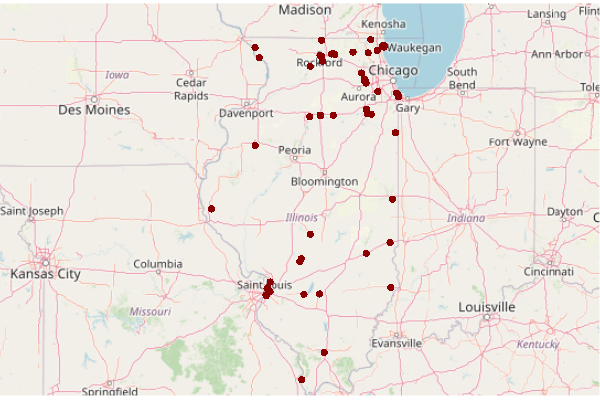
Cleanups in My Community sites in Illinois

Subset Superfund Sites

The Superfund sites in this list are the ones where a URL is provided to an information page in the superfund = cimc[cimc$Superfund.Link.CSV != "",]

Subset only the Superfund sites.

superfund = cimc[cimc$Superfund.Link.CSV != "",]

plot(basemap)

plot(st_transform(st_geometry(superfund), osm()@projargs), col="darkred", pch=16, add=T)

Load Demographic, Cancer, and Toxics Releases Data

The prepared geospatial data described earlier can be loaded using the st_read() function from the sf library. The stringsAsFactors = F parameter permits an internal representation of text names in the objects that can be more conveniently used in analysis.

toxics = st_read("2021-minn-toxics-facilities.geojson", stringsAsFactors = F, quiet=T)

zip.codes = st_read("2021-minn-toxics-zip.geojson", stringsAsFactors = F, quiet=T)

Analyze the Data

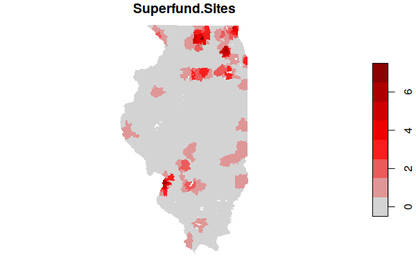
Find Affected ZIP Codes

For our initial analysis we look for ZIP Codes that are near brownfields.

The sf_use_s2() function call will instruct st_buffer() to use the s2 spherical geometry package for geographical coordinate operations.
To model the areas of influence, we create circular buffers around each site using the st_buffer() function.
The dist=8000 parameter specifies the radius of each buffer, where 8000 kilometers is roughly five miles. Note that this buffer size is an arbitrary compromise since Superfund sites vary in size, toxicity, and contaminant transport mechanism.
st_intersects() returns a list containing the feature number(s) for the buffers that intersect with each ZIP Code (if any).
The lengths() function returns a vector of the number of entries in each intersection list element. This provides the number of Superfund sites at each ZIP Code.

sf_use_s2(T)

buffers = st_buffer(superfund, dist=8000)

intersections = st_intersects(zip.codes, buffers)

zip.codes$Superfund.Sites = lengths(intersections)

plot(zip.codes["Superfund.Sites"], border=NA, pal=colorRampPalette(c("lightgray", "red", "darkred")))

Numer of Superfund sites affecting ZIP Codes in Illinois

You can get a list of the most affected ZIP Codes by ordering the data frame by the number of sites and displaying the head() six entries.

zip.codes = zip.codes[order(zip.codes$Superfund.Sites, decreasing=T),]

head(st_drop_geometry(zip.codes[,c("Name", "Superfund.Sites")]))

	    Name	Superfund.Sites
	404 61016               7
	67  60103               6
	126 60185               6
	872 62040               6
	52  60083               5
	88  60134               5

Find Statewide Demographics

To be able to evaluate distinct demographic characteristics of areas, we use statewide values for context from the US Census Bureau.

data.census.gov has overall profile pages for areas that you can find by typing in the name of the area and choosing the profile page when the form offers suggestion.

Getting statewide demographic information from data.census.gov

Find Demographic Characteristics of Areas around Superfund Sites

We can use sum() and weighted.mean() functions to get the corresponding values for comparison to state values. weighted.mean() is used rather than mean() so that the mean reflects the overall population affected without being biased by sparsely-populated ZIP Code areas.

superzip = zip.codes[zip.codes$Superfund.Sites > 0,]

sum(superzip$Total.Population, na.rm=T)

	[1] 4603910

weighted.mean(superzip$Median.Household.Income, weights = superzip$Total.Population, na.rm=T)

	[1] 68222.72

weighted.mean(superzip$Median.Age, weights = superzip$Total.Population, na.rm=T)

	[1] 41.25802

weighted.mean(superzip$Percent.Bachelors.Degree, weights = superzip$Total.Population, na.rm=T)

	[1] 17.02423

weighted.mean(superzip$Percent.Homeowners, weights = superzip$Total.Population, na.rm=T)

	[1] 73.64778

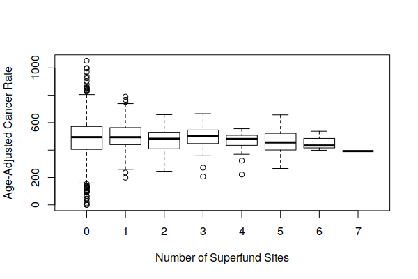
Compare Cancer Rates

Comparing cancer rates around Superfund sites with the state as a whole, there is no significant difference. This value is for all cancers, and rates for specific cancers may be different.

weighted.mean(zip.codes$Age.Adjusted.Rate, weights = zip.codes$Total.Population, na.rm=T)

	[1] 484.938

weighted.mean(superzip$Age.Adjusted.Rate, weights = zip.codes$Total.Population, na.rm=T)

	[1] 485.5583

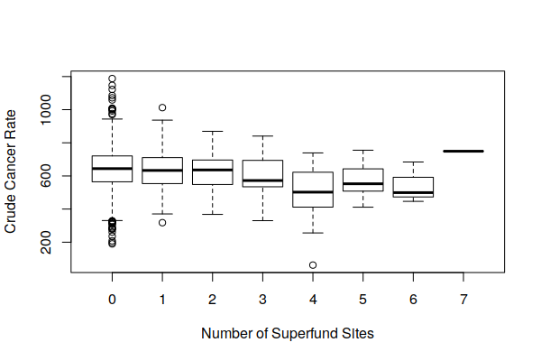
However, when viewing boxplot() of the distribution of both crude cancer rates and age-adjusted cancer rates by number of Superfund sites, we see that cancer rates vary widely around Superfund sites, and the number of Superfund sites does not appear to be a major factor affecting cancer rates.

boxplot(Age.Adjusted.Rate ~ Superfund.Sites, data = zip.codes, 
	xlab="Number of Superfund Sites", ylab="Age-Adjusted Cancer Rate")

Age-adjusted cancer rates by ZIP Code vs. number of Superfund sites

boxplot(Estimated.Rate ~ Superfund.Sites, data = zip.codes, 
	xlab="Number of Superfund Sites", ylab="Crude Cancer Rate")

Crude cancer rates by ZIP Code vs. number of Superfund sites

Brownfields vs. Active Plants

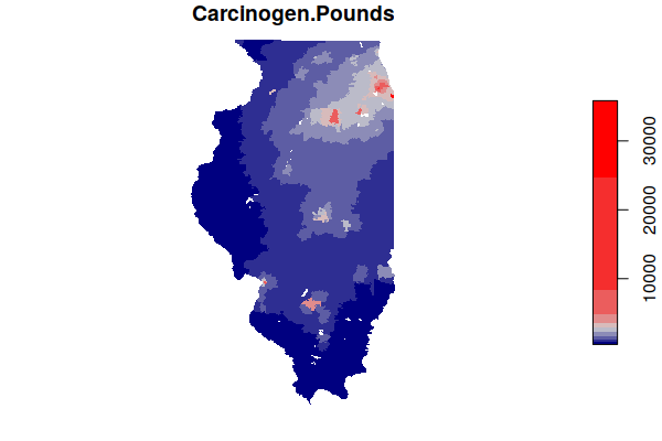
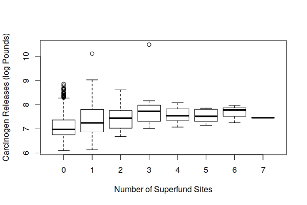
Because industrial sites tend to be clustered together (agglomeration), we might assume that brownfields would often be located near active industrial sites. A boxplot() of carcinogenic releases by active facilities and number of Superfund sites offers some confirmation of this, with areas around Superfund sites also tending to also be affected by higher carcinogenic releases from adjacent active industrial facilities.

This presents a significant confounder in trying to evaluate the negative cancer effect of brownfields on adjacent communities.

boxplot(log(Carcinogen.Pounds) ~ Superfund.Sites, data = zip.codes,
	xlab="Number of Superfund Sites", ylab="Carcinogen Releases (log Pounds)")

Box plot comparing levels of carcinogenic releases by active facilities vs. number of Superfund sites in the area

Identifying Potential High-Impact Superfund Sites

By taking a area weighted mean of cancer rates and demographic variables using the buffers around Superfund sites, we can identify sites that may have the highest impact on surrounding communities.

Note that the st_interpolate_aw() function may take awhile to complete.

zip.numeric = Filter(is.numeric, zip.codes)

supersites = st_interpolate_aw(zip.numeric, buffers, extensive=F, keep_NA=T)

supersites = cbind(supersites, st_drop_geometry(buffers))

supersites = supersites[order(supersites$Age.Adjusted.Rate, decreasing=T),]

head(st_drop_geometry(supersites[,c("Cleanup.Name", "City.Name",
	"Median.Household.Income", "Age.Adjusted.Rate")]))

				       Cleanup.Name           City.Name
	37                         ILADA ENERGY CO. EAST CAPE GIRARDEAU
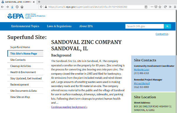
	9                          SANDOVAL ZINC CO            SANDOVAL
	16 CROSS BROTHERS PAIL RECYCLING (PEMBROKE)   PEMBROKE TOWNSHIP
	7                              HEGELER ZINC            DANVILLE
	51                   OTTAWA RADIATION AREAS              OTTAWA
	42                    CIRCLE SMELTING CORP.          BECKEMEYER

	   Median.Household.Income Age.Adjusted.Rate
	37                39602.23          713.6692
	9                 48745.67          626.7814
	16                40139.07          594.1077
	7                 51946.86          573.3866
	51                56961.84          561.6495
	42                67960.75          547.5869

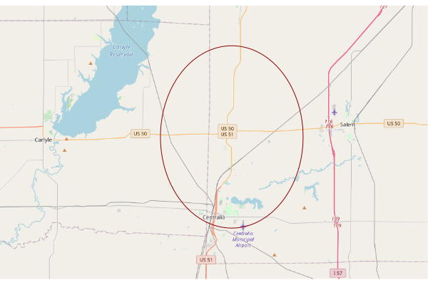
Site Location Map

This creates a map of the third site in the list (index 2) using OpenStreetMap tiles that is zoomed out enough to give some context of where the site is located in the state.

site = supersites[2,]

upperLeft = c(site$Latitude + 0.15, site$Longitude - 0.3)

lowerRight = c(site$Latitude - 0.15, site$Longitude + 0.3)

sitebase = openmap(upperLeft = upperLeft, lowerRight = lowerRight)

plot(sitebase)

plot(st_transform(st_geometry(site), osm()@projargs), border="darkred", col=NA, add=T)

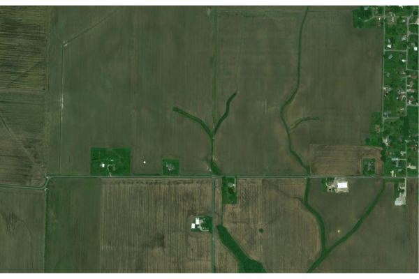
Aerial Image

You can create get an aerial image of the site using using Bing map tiles with the openmap() function from the OpenStreetMap library.

upperLeft = c(site$Latitude + 0.005, site$Longitude - 0.01)

lowerRight = c(site$Latitude - 0.005, site$Longitude + 0.01)

sitebase = openmap(upperLeft = upperLeft, lowerRight = lowerRight, type="bing")

plot(sitebase)

plot(st_transform(st_geometry(site), osm()@projargs), border="darkred", col=NA, add=T)

Sandovol Zinc Superfund site aerial view (Bing)

Viewing Neighborhood Demographics

You can view the demographic information and cancer rates by viewing all fields for the site.

print(site)

  Median.Household.Income Median.Age Percent.Bachelors.Degree
9                48745.67    42.2448                 8.727277

  Percent.Homeowners Estimated.Rate Age.Adjusted.Rate CARCINOGEN.POUNDS
9            76.4792       778.5343          626.7814                NA

                                                  Superfund.Link.CSV
9 https://cumulis.epa.gov/supercpad/cursites/csitinfo.cfm?id=0500360

  ECHO.Link.CSV Response.Link.CSV
9                                
                                                           RE.Powering.CSV
9 https://ofmpub.epa.gov/apex/cimc/f?p=CIMC:REPOWER:::::P6_REFERENCE:81630
                                                                                          FRS.Link.CSV
9 https://ofmpub.epa.gov/frs_public2/fii_query_detail.disp_program_facility?p_registry_id=110018406125
                                                                         Map.Site.CSV
9 https://ofmpub.epa.gov/apex/cimcf?p=CIMC:MAP:::::P71_GEOSEARCH:38.613061 -89.108251

Viewing EPA Information on the Site

The cleanups data contains URLs to EPA information web pages for the sites. The Superfund.Link.CSV points to the Superfund web site home page for the site, which, in turn, contains links to other pages that provide information like history, description, current status, and site contaminants.